01. Probability toolkit¶
Where this fits
Prerequisites: none. This is the first technical chapter. Used later by: Chapter 2 (learning from examples), Chapter 9 (Hoeffding's inequality), Chapters 10, 11, 15 and 17, and every chapter after them. Purpose: give you the exact vocabulary needed to read the paper's sentences of the form "with probability at least \(1-\delta\), …", so that you can say what is random, what is fixed, and why an average over many independent draws can be trusted.
The problem this chapter solves¶
PAPER §4.1, p. 4 The paper's central tool is its Eq. (1). It is a promise about a trained model: the model's average error on new text is at most its average error on the training text, plus a penalty. The promise is said to hold "with probability at least \(1-\delta\)". It also requires that the training documents were sampled independently. Every later bound in the paper (Eq. (3) in §4.4 and Eq. (8) in Appendix A.3) has the same form.
MY EXPLANATION You cannot read a sentence like that without a few precise ideas. Three questions need answers.
- Probability of what? Something in the sentence must be random. What is it? And what stays fixed?
- What does "independently" mean? And why does the paper insist on it?
- Why should an average over a sample tell us anything about an average over everything?
This chapter builds the answers from nothing, using dice and opinion polls. By the end you will be able to take any "with probability at least \(1-\delta\)" sentence and say exactly what it promises, and what it does not.
Notation in this chapter
In this chapter \(n\) is a generic number of draws and \(X\) is a generic random number. From Chapter 2 on, the paper's notation takes over (see the notation table): \(X_j\) is a training document, \(m\) is the number of training documents, and \(n\) is reserved for the size of a subsample. Here the Greek letter \(\sigma\) (sigma) is a standard deviation. The paper also writes \(\sigma(i)\) for something unrelated: the index of a subsampled document (Chapter 17).
Intuition (and where the analogy breaks)¶
Everything in this section is MY EXPLANATION.
Imagine a country with millions of voters. You want to know what fraction of them support a new law. Asking everyone is impossible. So you ask 1,000 voters chosen at random, and you report the fraction of "yes" answers in your sample.
Why should this work? Each randomly chosen voter is a fair representative of the whole country. Some samples will contain a few too many "yes" voters. Others will contain too few. With 1,000 voters these accidents mostly cancel. The sample fraction lands close to the true fraction, usually.
"Usually" is the key word. It is possible, though fantastically unlikely, to pick 1,000 people who all say "yes". No method that looks at only part of a population can promise to be right every time. The best it can promise is to be right most of the time.
That is why a pollster reports something like "the margin of error is 3.1 percentage points, 19 times out of 20" (for a poll of 1,000 people; the worked example computes this number). "19 times out of 20" is a promise about the polling method. If many pollsters each ran the same method on fresh random samples, about 19 in 20 of them would land within the margin. It is not a promise about any one finished poll. A finished poll either landed within the margin or it did not.
The paper's bounds work the same way. The poll maps onto the paper like this:
- a voter ↔ a training document;
- a voter's answer ↔ the model's error on that document (a number, called the loss; Chapter 2);
- the fraction of "yes" among all voters ↔ the model's average error over all possible documents (Chapter 2 calls this the expected risk);
- the fraction of "yes" in the sample ↔ the model's average error on its training documents (Chapter 2: the empirical risk);
- "19 times out of 20" ↔ "with probability at least \(1-\delta\)" with \(\delta = 0.05\).
Where it breaks:
- The question is chosen after seeing the answers. A pollster fixes the question before asking anyone. A learning algorithm picks its model after looking at the training data. The "question" depends on the answers, and this can make the sample look misleadingly good. Chapter 10 shows the damage and the repair.
- Answers are not just 0 or 1. Poll answers are yes or no. A model's error on a document can be any non-negative number, and the error measure the paper cares about most has no upper limit at all. Chapter 16 shows how the paper squeezes it into a bounded range.
- Real polls sample without replacement. A pollster never asks the same person twice. The paper's theory instead treats documents as independent draws. This chapter shows that these are different things (and how much the difference matters); Chapters 15 and 17 return to it.
Precise definition¶
Everything in this section is MY EXPLANATION (standard textbook material) unless tagged otherwise.
We work with discrete experiments: ones whose possible results can be listed as a finite list, or as an endless list numbered 1, 2, 3, … ("countably many"). That is enough for the whole paper. A document is a finite string of characters, and all finite strings can be listed one after another (shortest first, alphabetically within each length). The one continuous object we need, the normal distribution, gets its own subsection.
Experiments, outcomes and events¶
An experiment is any procedure whose result is not known in advance. Rolling a die is an experiment. So is "pick 10,000 documents at random from a large collection".
An outcome is one possible result of the experiment. The set of all outcomes is the sample space, written \(\Omega\) (capital omega). For one roll of a die, \(\Omega=\{1,2,3,4,5,6\}\). For ten rolls, an outcome is a list of ten numbers such as \((3,1,6,6,2,5,4,1,1,3)\), and \(\Omega\) contains every such list.
An event is a set of outcomes. Think of it as a yes/no question about the result. "The roll is even" is the event \(A=\{2,4,6\}\). We say that \(A\) happens if the actual outcome lies in \(A\).
Events combine like sets. "\(A\) or \(B\)" is the union \(A\cup B\). "\(A\) and \(B\)" is the intersection \(A\cap B\). "Not \(A\)" is the complement \(A^c\), all outcomes outside \(A\). Two events are disjoint if they cannot both happen, that is, \(A\cap B=\varnothing\) (the empty set).
Probability¶
A probability is a rule \(\Pr\) that gives every event \(A\) a number \(\Pr(A)\) and obeys three rules, called the axioms:
- \(\Pr(A)\ge 0\) for every event \(A\).
- \(\Pr(\Omega)=1\). (Something certainly happens.)
- Additivity. If \(A_1, A_2, \dots\) are disjoint events, then \(\Pr(A_1\cup A_2\cup\cdots)=\Pr(A_1)+\Pr(A_2)+\cdots\).
A note on notation: we always write "\(\Pr\)" (short for "probability") for the probability of an event. The single letter \(P\) is kept for something else that the paper uses: a weighting of models, \(P(h)\), which appears at the end of this chapter and is made precise in Chapter 11.
For a discrete experiment, it is enough to give each outcome \(\omega\) (lower-case omega) a weight \(p(\omega)\ge0\), with all weights adding up to 1. The probability of an event is then the total weight of its outcomes:
A fair die gives each face weight \(1/6\). So \(\Pr(\text{even}) = 3\cdot\frac16 = \frac12\).
Two consequences are used all the time. The complement rule: \(\Pr(A^c)=1-\Pr(A)\), because \(A\) and \(A^c\) are disjoint and together make up \(\Omega\). And monotonicity: if every outcome in \(A\) is also in \(B\), then \(\Pr(A)\le \Pr(B)\).
Going deeper: consequences of the axioms, proved
MY EXPLANATION Each step uses only the three axioms.
The empty event has probability 0. The sequence \(\varnothing,\varnothing,\varnothing,\dots\) consists of disjoint events (no outcome lies in any of them) whose union is \(\varnothing\). Axiom 3 gives \(\Pr(\varnothing)=\Pr(\varnothing)+\Pr(\varnothing)+\cdots\). A non-negative number equals an endless sum of copies of itself only if it is 0. So \(\Pr(\varnothing)=0\).
Finite additivity. For two disjoint events \(A,B\), use the sequence \(A,B,\varnothing,\varnothing,\dots\). Axiom 3 and \(\Pr(\varnothing)=0\) give \(\Pr(A\cup B)=\Pr(A)+\Pr(B)\). The same padding works for any finite number of events.
Complement rule. \(A\) and \(A^c\) are disjoint and \(A\cup A^c=\Omega\). Finite additivity and axiom 2 give \(\Pr(A)+\Pr(A^c)=1\).
Monotonicity. Suppose \(A\subseteq B\). Write \(B=A\cup(B\setminus A)\), where \(B\setminus A\) is the set of outcomes in \(B\) but not in \(A\). The two pieces are disjoint, so \(\Pr(B)=\Pr(A)+\Pr(B\setminus A)\ge \Pr(A)\) by axiom 1. With \(B=\Omega\) this also shows \(\Pr(A)\le1\).
The weight construction obeys the axioms. Define \(\Pr(A)=\sum_{\omega\in A}p(\omega)\) with \(p(\omega)\ge0\) and \(\sum_{\omega\in\Omega}p(\omega)=1\). Axiom 1 holds because a sum of non-negative weights is non-negative. Axiom 2 is the normalisation. For axiom 3, every outcome of \(\bigcup_k A_k\) lies in exactly one \(A_k\) (they are disjoint), so the total weight of the union can be computed piece by piece: \(\sum_{\omega\in\cup_k A_k}p(\omega)=\sum_k\sum_{\omega\in A_k}p(\omega)\). Re-grouping is allowed because all terms are non-negative, and the order of summation does not change a sum of non-negative terms.
Random variables and distributions¶
A random variable is a number computed from the outcome. Formally it is a function \(X\) that turns each outcome \(\omega\) into a number \(X(\omega)\). Examples: the number of pips on a die; the mean of ten rolls; a model's error on a randomly drawn document.
A random variable is not "random" by itself. It is a fixed recipe. The randomness comes from the outcome that is fed into it. We write random variables with capital letters (\(X\)) and particular values with lower-case letters (\(x\)).
A useful special case is the indicator of an event \(A\), written \(\mathbf 1[A]\). It equals 1 if \(A\) happens and 0 if not. It turns a yes/no question into a number. A poll answer is an indicator: 1 for "yes", 0 for "no".
The distribution of a random variable \(X\) is the list of values it can take, together with the probability of each value. We write \(\Pr(X=x)\) as shorthand for the probability of the event "\(X\) equals \(x\)", which is the set of outcomes \(\{\omega : X(\omega)=x\}\). For a fair die, each value \(1,\dots,6\) has probability \(1/6\).
Two random variables with the same distribution are called identically distributed. The first and the second roll of a die are identically distributed, even though they are different rolls.
Expectation¶
The expectation of \(X\) (also expected value or mean) is the probability-weighted average of its values:
For a fair die, \(\mathbb E[X]=(1+2+3+4+5+6)/6=3.5\) pips. The die can never show 3.5. The expectation is the balance point of the distribution, and (as the law of large numbers below shows) the long-run average of many rolls.
For an indicator, \(\mathbb E[\mathbf 1[A]] = 1\cdot \Pr(A)+0\cdot \Pr(A^c)=\Pr(A)\). Every probability is the expectation of an indicator. This small fact powers Markov's inequality below.
Two properties of expectation are used everywhere:
- Linearity of expectation. \(\mathbb E[aX+bY]=a\,\mathbb E[X]+b\,\mathbb E[Y]\) for any random variables \(X,Y\) and any constants \(a,b\). This holds always, even when \(X\) and \(Y\) depend strongly on each other. It extends to sums of many terms: \(\mathbb E[X_1+\cdots+X_n]=\mathbb E[X_1]+\cdots+\mathbb E[X_n]\).
- Monotonicity. If \(X\le Y\) for every outcome, then \(\mathbb E[X]\le\mathbb E[Y]\).
PAPER §4.1, p. 4 The paper defines the expected risk of a model \(h\) as the expectation of its empirical risk, \(R(h)=\mathbb E[\hat R(h)]\). Here \(\hat R(h)=\frac1m\sum_{j=1}^m R(h,X_j)\) is the average error of the model over the \(m\) training documents \(X_1,\dots,X_m\), and \(R(h,X)\) is its error on one document \(X\). (Chapter 2 defines these terms properly.)
MY EXPLANATION Linearity turns this into something more intuitive. Hold the model \(h\) fixed. If every training document has the same distribution as a single random document \(X\), then
So the expected risk is the expected error on one fresh document. This step needs only "identically distributed". It does not need independence.
Going deeper: expectation of a function, linearity and monotonicity, proved
MY EXPLANATION
Two equivalent formulas. For a discrete experiment we can also average over outcomes: \(\mathbb E[X]=\sum_\omega X(\omega)\,p(\omega)\). This agrees with the definition above. Group the outcomes by the value \(x\) that \(X\) gives them:
When \(X\) can take infinitely many values we require \(\sum_x |x|\,\Pr(X=x)<\infty\) ("absolute convergence"). Then the order of summation does not matter and the regrouping above is legal. Every loss the paper's bounds use is confined to a bounded interval (Chapter 16), so the expectation always exists there.
Expectation of a function. The same grouping with \(g(X(\omega))\) in place of \(X(\omega)\) gives \(\mathbb E[g(X)]=\sum_x g(x)\,\Pr(X=x)\). For a pair of random variables, \(\mathbb E[g(X,Y)]=\sum_{x,y}g(x,y)\,\Pr(X=x,Y=y)\), where \(\Pr(X=x,Y=y)\) is the probability that both happen.
Linearity. Both \(X\) and \(Y\) are functions on the same sample space. So
Nothing about how \(X\) and \(Y\) relate was used. That is why linearity needs no independence. Applying the two-term rule repeatedly (induction on \(n\)) gives the rule for \(n\) terms. A constant \(c\) has \(\mathbb E[c]=c\sum_\omega p(\omega)=c\).
Monotonicity. If \(X(\omega)\le Y(\omega)\) for every \(\omega\), then \(X(\omega)p(\omega)\le Y(\omega)p(\omega)\) term by term (because \(p(\omega)\ge0\)). Adding up gives \(\mathbb E[X]\le\mathbb E[Y]\).
Variance and standard deviation¶
The expectation says where a random variable is centred. The variance says how far it typically strays from that centre.
The variance of \(X\) is the expected squared distance from its mean:
Squaring makes all distances positive. It also changes the units: if \(X\) is in pips, the variance is in pips². The standard deviation is the square root, \(\sqrt{\operatorname{Var}[X]}\), which is back in the units of \(X\). We write \(\mu\) (mu) for a mean and \(\sigma\) (sigma) for a standard deviation, so \(\sigma^2\) is a variance.
For a fair die the variance is \(35/12\approx2.916667\) pips², and the standard deviation is about \(1.707825\) pips.
Two rules help with calculations. First, \(\operatorname{Var}[X]=\mathbb E[X^2]-(\mathbb E[X])^2\). Second, shifting does not change the spread and scaling multiplies it: \(\operatorname{Var}[aX+b]=a^2\operatorname{Var}[X]\).
Going deeper: the variance formulas, and the die's variance step by step
MY EXPLANATION Write \(\mu=\mathbb E[X]\), a constant.
Shortcut formula. Expand the square and use linearity:
Shift and scale. \(aX+b\) has mean \(a\mu+b\), so \((aX+b)-(a\mu+b)=a(X-\mu)\). Squaring and taking expectations gives \(\operatorname{Var}[aX+b]=a^2\,\mathbb E[(X-\mu)^2]=a^2\operatorname{Var}[X]\).
Sign. A variance is the expectation of a square, so it is \(\ge0\) by monotonicity. It is 0 exactly when \(X=\mu\) on every outcome that has positive probability.
The die. \(\mathbb E[X^2]=(1+4+9+16+25+36)/6=91/6\). So \(\operatorname{Var}[X]=\frac{91}{6}-\big(\frac72\big)^2=\frac{182}{12}-\frac{147}{12}=\frac{35}{12}\approx2.916667\) pips², and the standard deviation is \(\sqrt{35/12}\approx1.707825\) pips. The script checks these with exact fractions.
Independence¶
Two events \(A\) and \(B\) are independent if
Intuitively, learning that \(B\) happened does not change how likely \(A\) is. (The next subsections make this exact.)
Two random variables \(X\) and \(Y\) are independent if \(\Pr(X=x,\,Y=y)=\Pr(X=x)\,\Pr(Y=y)\) for every pair of values \(x,y\). Several random variables \(X_1,\dots,X_n\) are (mutually) independent if the same product rule holds for all of them at once:
Two different rolls of a die are independent. A roll and the event "that same roll is even" are not.
Independence buys a product rule for expectations: if \(X\) and \(Y\) are independent, then \(\mathbb E[XY]=\mathbb E[X]\,\mathbb E[Y]\). Without independence this fails. For example, with \(Y=X\) it would claim \(\mathbb E[X^2]=(\mathbb E[X])^2\), which is false whenever the variance is positive.
The product rule makes variances add up. Define the covariance of \(X\) and \(Y\) as \(\operatorname{Cov}(X,Y)=\mathbb E\big[(X-\mathbb E[X])(Y-\mathbb E[Y])\big]\). It is positive when \(X\) and \(Y\) tend to be above their means together, and negative when one tends to be high while the other is low. In general,
Independent variables have covariance 0, so for them \(\operatorname{Var}[X+Y]=\operatorname{Var}[X]+\operatorname{Var}[Y]\).
The reverse is false: covariance 0 does not imply independence. The script's example: let \(U\) be \(-1\), \(0\) or \(1\) with equal probability, and \(W=U^2\). Then \(\operatorname{Cov}(U,W)=0\), yet \(\Pr(U=0,W=0)=1/3\) while \(\Pr(U=0)\,\Pr(W=0)=1/9\). Knowing \(U\) tells you \(W\) exactly.
PAPER §4.2, p. 5 In its note on satisfying the i.i.d. assumption, the paper stresses that whether samples from a set are independent depends on how we sample from the set, not on what the set contains. A set of very similar documents can still be sampled independently.
MY EXPLANATION The definition above agrees. Independence is a property of the joint probabilities of the draws, which the sampling procedure creates. It says nothing about the content of the items. Chapter 15 examines what this does and does not buy the paper.
Going deeper: the product rule for independent variables, covariance, and the variance of a sum
MY EXPLANATION
Product rule. Use the expectation of a function of the pair, \(g(x,y)=xy\), then independence, then factor the double sum:
The same steps with \(f(x)g(y)\) in place of \(xy\) show \(\mathbb E[f(X)g(Y)]=\mathbb E[f(X)]\,\mathbb E[g(Y)]\) for any functions \(f,g\).
Covariance shortcut. With \(\mu_X=\mathbb E[X]\) and \(\mu_Y=\mathbb E[Y]\), expanding and using linearity gives \(\operatorname{Cov}(X,Y)=\mathbb E[XY]-\mu_X\mu_Y\). Under independence this is \(\mu_X\mu_Y-\mu_X\mu_Y=0\). Variables with covariance 0 are called uncorrelated.
Variance of a sum. Let \(Y_i=X_i-\mathbb E[X_i]\). Then \(\big(\sum_i Y_i\big)^2=\sum_i\sum_j Y_iY_j\). Taking expectations term by term (linearity):
If the variables are pairwise uncorrelated (for example, independent), the second sum vanishes and variances add. With \(n=2\) this is the formula \(\operatorname{Var}[X+Y]=\operatorname{Var}[X]+\operatorname{Var}[Y]+2\operatorname{Cov}(X,Y)\) from the main text, because the pairs \((1,2)\) and \((2,1)\) both contribute \(\operatorname{Cov}(X,Y)\).
Uncorrelated but dependent. \(U\) uniform on \(\{-1,0,1\}\), \(W=U^2\). Then \(\mathbb E[U]=0\) and \(UW=U^3\), whose expectation is also 0 by symmetry. So \(\operatorname{Cov}(U,W)=\mathbb E[UW]-\mathbb E[U]\,\mathbb E[W]=0\). But the event \(U=0\) forces \(W=0\), so \(\Pr(U=0,W=0)=\Pr(U=0)=1/3\), while \(\Pr(U=0)\Pr(W=0)=\frac13\cdot\frac13=\frac19\).
Mutual independence covers sub-collections. If the product rule holds for all \(n\) variables, sum both sides over all values of \(X_3,\dots,X_n\). Each factor \(\sum_{x_k}\Pr(X_k=x_k)\) equals 1, leaving \(\Pr(X_1=x_1,X_2=x_2)=\Pr(X_1=x_1)\Pr(X_2=x_2)\). So mutually independent variables are also pairwise independent, and therefore pairwise uncorrelated.
Independent and identically distributed (i.i.d.)¶
Random variables \(X_1,\dots,X_n\) are i.i.d. (independent and identically distributed) if they are mutually independent and all have the same distribution. Repeated rolls of one die are i.i.d. Voters drawn with replacement (defined below) are i.i.d.
PAPER §4.1, p. 4 The paper's Eq. (1) assumes the training documents \(X_1,\dots,X_m\) are sampled independently, each from the same source of documents. MY EXPLANATION That is the i.i.d. assumption. Chapter 15 discusses what "the same source" means for a real text collection.
Conditional probability¶
The conditional probability of \(A\) given \(B\) is
Read it as "the probability of \(A\), if we already know that \(B\) happened". The recipe: throw away every outcome outside \(B\), then rescale the remaining outcomes so that their probabilities add up to 1 again.
Example: roll a fair die and let \(B\) = "even", \(A\) = "the roll is 6". Then \(\Pr(A\mid B)=(1/6)/(1/2)=1/3\). Knowing the roll is even triples the chance of a 6.
Now the intuition behind independence is exact: when \(\Pr(B)>0\), the events \(A\) and \(B\) are independent exactly when \(\Pr(A\mid B)=\Pr(A)\). (Divide both sides of \(\Pr(A\cap B)=\Pr(A)\Pr(B)\) by \(\Pr(B)\).)
One more rule, the law of total probability, splits a probability into cases. If the events \(B_1,B_2,\dots\) are disjoint and together cover \(\Omega\), then
A consequence used in Chapter 17: if \(\Pr(A\mid B_k)\le\delta\) in every case \(k\), then \(\Pr(A)\le\delta\). A guarantee that holds for every fixed value of something random also holds when that something is random.
Conditional expectation¶
The conditional expectation of \(Y\) given \(X=x\) is the average of \(Y\) over only those outcomes where \(X=x\):
This gives one number for each value \(x\). Plugging the random \(X\) into that recipe gives a new random variable, written \(\mathbb E[Y\mid X]\). It is a function of \(X\).
The tower rule says that averaging these group averages, weighted by how likely each group is, gives back the overall average:
Example: roll two dice, \(X_1\) and \(X_2\), and let \(Y=X_1+X_2\). Given \(X_1=x\), the average of \(Y\) is \(x+3.5\), because the second die does not care about the first. So \(\mathbb E[Y\mid X_1]=X_1+3.5\). Its expectation is \(3.5+3.5=7\), which is \(\mathbb E[Y]\), as the tower rule promises.
You may condition on any random object, not only on a number. In particular you may condition on an entire random dataset.
PAPER App. A.3, p. 14 The paper does exactly this. It estimates the training error on a random subsample of the training set, and it analyses the subsample "considering X fixed", where \(X\) denotes the whole training set. It also uses the fact that, given the training set, the subsample's average error equals on average the training set's average error.
MY EXPLANATION By the tower rule, that fact implies that the subsample's average error has the same expectation as the full training error. The law of total probability then turns a guarantee for every fixed training set into a guarantee overall. Chapter 17 carries out this argument in full.
Going deeper: the law of total probability and the tower rule, proved
MY EXPLANATION
Law of total probability. Let \(B_1,B_2,\dots\) be disjoint, cover \(\Omega\), and have \(\Pr(B_k)>0\). The pieces \(A\cap B_k\) are disjoint and their union is \(A\). Additivity and the definition of conditional probability give
If every \(\Pr(A\mid B_k)\le\delta\), then \(\Pr(A)\le\delta\sum_kP(B_k)=\delta\cdot1=\delta\). (Cases with \(\Pr(B_k)=0\) contribute nothing to \(\Pr(A)\) and can be dropped.)
Tower rule. Let \(g(x)=\mathbb E[Y\mid X=x]\), so \(\mathbb E[Y\mid X]=g(X)\). Then
Line 1 uses the expectation of a function of \(X\) and the definition of \(g\). Line 2 first uses \(\Pr(Y=y\mid X=x)\Pr(X=x)=\Pr(X=x,Y=y)\) (the definition of conditional probability), then swaps the two sums (allowed under absolute convergence), then applies the law of total probability with the cases \(B_x=\{X=x\}\).
Independence. If \(X\) and \(Y\) are independent then \(\Pr(Y=y\mid X=x)=\Pr(Y=y)\), so \(\mathbb E[Y\mid X=x]=\mathbb E[Y]\) for every \(x\). This was used in the two-dice example.
Probabilities are a special case. With \(Y=\mathbf 1[A]\), the conditional expectation is \(\mathbb E[\mathbf 1[A]\mid X=x]=\Pr(A\mid X=x)\), and the tower rule becomes the law of total probability.
The normal (Gaussian) distribution¶
Some random quantities can take any real value: a height, a measurement error. For these, the probability of any single exact value is 0. Probabilities come instead from a density \(f(x)\). The probability of an interval is the area under the curve \(f\) over that interval.
The most important density is the normal (Gaussian) distribution with mean \(\mu\) and variance \(\sigma^2\), written \(\mathcal N(\mu,\sigma^2)\):
Here \(\pi\) is the circle constant and \(\exp(u)=e^u\) is the exponential function, which Chapter 3 introduces properly. For now you only need that \(\exp(-u)\) shrinks quickly towards 0 as \(u\) grows. So \(f\) is a symmetric bell curve, highest at \(\mu\), whose width is set by \(\sigma\). A normal variable with \(\mu=0\) and \(\sigma=1\) is called standard and is usually written \(Z\). About 95 % of its area lies within 1.96 of the centre: the script computes \(\Pr(|Z|\ge1.96)=0.05000\).
Why it appears here. First, the histograms of sample means in the worked example look like bell curves. (A theorem called the central limit theorem explains why; we do not need it.) Second, Chapters 8 and 18 build random matrices whose entries are drawn from normal distributions. The paper's bounds do not use normal approximations. They need statements that are exactly true for every sample size, which is why this chapter ends with inequalities.
Going deeper: the normal density has total area 1, mean mu and variance sigma squared
MY EXPLANATION For a continuous random variable with density \(f\), expectations are integrals: \(\mathbb E[g(X)]=\int_{-\infty}^{\infty}g(x)f(x)\,dx\).
Standardise. Substitute \(x=\mu+\sigma z\), so \(dx=\sigma\,dz\). Then every claim reduces to integrals of \(e^{-z^2/2}\), and \(X=\mu+\sigma Z\) where \(Z\) has density \(\frac{1}{\sqrt{2\pi}}e^{-z^2/2}\).
Total area. Let \(I=\int_{-\infty}^{\infty}e^{-z^2/2}\,dz\). Multiply two copies and switch to polar coordinates \(z=r\cos\theta\), \(w=r\sin\theta\), for which the area element is \(dz\,dw=r\,dr\,d\theta\):
Since \(I>0\), \(I=\sqrt{2\pi}\), so the density integrates to 1. (Skipped: the justification that this improper double integral may be computed in either coordinate system. It holds because the integrand is non-negative, by Tonelli's theorem.)
Mean. \(z\,e^{-z^2/2}\) is an odd function (it changes sign when \(z\) does), and it is integrable because \(e^{-z^2/2}\) decays faster than any power of \(z\). So \(\mathbb E[Z]=0\) and \(\mathbb E[X]=\mu+\sigma\cdot0=\mu\).
Variance. Integrate by parts with \(u=z\) and \(dv=z\,e^{-z^2/2}dz\), so \(v=-e^{-z^2/2}\):
Dividing by \(\sqrt{2\pi}\) gives \(\mathbb E[Z^2]=1\), so \(\operatorname{Var}[Z]=1-0^2=1\) and \(\operatorname{Var}[X]=\sigma^2\operatorname{Var}[Z]=\sigma^2\).
Populations, samples and the sample mean¶
A population is the collection of items we draw from. In this chapter it is a finite list of \(N\) items, each carrying a number \(a_1,\dots,a_N\): voters with their answers, or documents with a model's error on each. The population mean is \(\mu=\frac1N\sum_{k=1}^N a_k\). The population variance is \(\sigma^2=\frac1N\sum_{k=1}^N(a_k-\mu)^2\). (Chapter 15 widens "population" to an unlimited source of documents.)
These are exactly the mean and variance of one item drawn at random with every item equally likely. If \(D\) is the number on that item, then \(\mathbb E[D]=\mu\) and \(\operatorname{Var}[D]=\sigma^2\).
Now draw \(n\) items and record their numbers \(X_1,\dots,X_n\). The sample mean is
The sample mean is a random variable: it depends on which items were drawn. If \(X_1,\dots,X_n\) are i.i.d. with mean \(\mu\) and variance \(\sigma^2\), then
In words: the sample mean is right on average, and its typical error shrinks like \(1/\sqrt n\). To halve the typical error you need four times as many draws.
Going deeper: mean and variance of the sample mean, proved
MY EXPLANATION
Mean. By linearity, \(\mathbb E[\bar X_n]=\frac1n\sum_{i=1}^n\mathbb E[X_i]=\frac1n\cdot n\mu=\mu\). Only "each \(X_i\) has mean \(\mu\)" was used.
Variance. By the scaling rule with \(a=1/n\), \(\operatorname{Var}[\bar X_n]=\frac1{n^2}\operatorname{Var}\big[\sum_iX_i\big]\). Independent variables are pairwise uncorrelated, so the variance of the sum is the sum of the variances, \(n\sigma^2\). Hence \(\operatorname{Var}[\bar X_n]=n\sigma^2/n^2=\sigma^2/n\).
Units. If each \(X_i\) is in pips, \(\sigma^2/n\) is in pips² and \(\sigma/\sqrt n\) is in pips.
What was really needed. Equal means, equal variances, and zero covariances. Full independence is more than enough. The next subsection shows what happens when the covariances are negative.
Sampling with and without replacement¶
There are two common ways to draw \(n\) items from a population of \(N\).
- Sampling with replacement. Draw an item uniformly at random, record it, put it back, and repeat. Each draw is uniform over all \(N\) items no matter what came before. So the draws are i.i.d. The same item can appear twice.
- Sampling without replacement. Draw an item, record it, and keep it out. No item appears twice. Each single draw, viewed on its own, is still uniform over all \(N\) items, so the draws are identically distributed. But they are not independent: if the first draw is item \(k\), the second draw cannot be item \(k\).
Without replacement, the sample mean varies less:
where \(\bar D_n\) is the mean of the \(n\) drawn numbers. The extra factor \(\frac{N-n}{N-1}\) is the finite-population correction. It equals 1 when \(n=1\). It equals 0 when \(n=N\): then you have drawn the whole population, and the sample mean is exactly \(\mu\). It is close to 1 when \(n\) is tiny compared with \(N\). Intuition: without replacement you never waste a draw on an item you have already seen.
PAPER §4.4, pp. 5–6 The paper estimates the training error on a random subsample of the training documents, drawing the indices with replacement.
PAPER App. A.3, p. 14 Its appendix allows the subsample to be drawn "with or without replacement".
Paper erratum E05: draws without replacement called I.I.D.
PAPER App. A.3, p. 14 The appendix describes the subsampled errors as I.I.D. random variables, and in parentheses as I.I.D. random variables sampled without replacement.
MY EXPLANATION The second phrase contradicts itself. Draws without replacement are identically distributed but dependent: in the script's population of 20 items, the second draw is item 1 with probability 0.0500, but with probability 0.0000 once the first draw was item 1. The paper's conclusion survives, because sampling without replacement concentrates at least as well as sampling with replacement (the variance formula above is one sign of this). But the inequality the paper applies is proved for independent variables, so the without-replacement case needs a separate theorem (Hoeffding 1963, Theorem 4), which the paper does not cite. The main text (§4.4) uses sampling with replacement, where no issue arises (and so does the authors' code, per erratum E05). Chapter 17 proves the missing step and simulates both schemes.
Going deeper: sampling without replacement, the negative covariance and the correction factor, proved
MY EXPLANATION Number the population positions \(1,\dots,N\) and let \(a_k\) be the number at position \(k\), with population mean \(\mu\) and population variance \(\sigma^2\) as defined above. Sampling \(n\) times without replacement produces an ordered list of distinct positions \((K_1,\dots,K_n)\). Every such list is equally likely, and there are \(N(N-1)\cdots(N-n+1)\) of them. The drawn numbers are \(D_i=a_{K_i}\).
Step 1: each draw on its own is uniform. Fix a slot \(i\) and a position \(k\). The lists with \(K_i=k\) are formed by filling the other \(n-1\) slots from the remaining \(N-1\) positions: \((N-1)(N-2)\cdots(N-n+1)\) lists. Dividing by the total gives \(\Pr(K_i=k)=1/N\). So every \(D_i\) has the distribution of a single uniform draw: \(\mathbb E[D_i]=\mu\) and \(\operatorname{Var}[D_i]=\sigma^2\).
Step 2: each pair is uniform over distinct pairs. For slots \(i\ne j\) and positions \(k\ne l\), the lists with \(K_i=k\) and \(K_j=l\) number \((N-2)\cdots(N-n+1)\), so \(\Pr(K_i=k,K_j=l)=\frac{1}{N(N-1)}\).
Step 3: the covariance is negative. Using Step 2,
The sum over all pairs \(k\ne l\) equals the sum over all pairs minus the diagonal \(k=l\):
(The deviations from the mean add up to zero, by the definition of \(\mu\).) Therefore \(\operatorname{Cov}(D_i,D_j)=-\sigma^2/(N-1)\).
Step 4: the variance of the sum. There are \(n\) variance terms and \(n(n-1)\) ordered pairs \(i\ne j\):
Dividing by \(n^2\) gives \(\operatorname{Var}[\bar D_n]=\frac{\sigma^2}{n}\cdot\frac{N-n}{N-1}\).
Checks. \(n=1\): factor 1. \(n=N\): factor 0. \(N\to\infty\) with \(n\) fixed: factor \(\to1\), recovering \(\sigma^2/n\).
Dependence. \(\Pr(K_2=k\mid K_1=k)=0\), but \(\Pr(K_2=k)=1/N\). So the draws are not independent.
With replacement, for contrast. Each \(K_i\) is uniform on \(\{1,\dots,N\}\) independently, so \(\Pr(K_1=k,K_2=l)=\frac1{N^2}=\Pr(K_1=k)\Pr(K_2=l)\) for all \(k,l\), including \(k=l\). The draws are i.i.d. and the covariance is 0.
Why the covariance is negative, in words. A high first draw removes a high value from the pool. The second draw then comes from a pool whose average is slightly lower. High and low draws therefore tend to alternate, and the average settles faster.
Fixed versus random¶
Here is a discipline that prevents most misreadings. Before you interpret any probability statement, sort every symbol in it into one of two bins.
- Random: it depends on the outcome of the experiment. Run the experiment again and it may change.
- Fixed: it was settled before the experiment, or it is a property of the world that the experiment does not change.
Take a concrete statement. Call it \(S\): "the mean of 10 rolls of a fair die lies strictly within 1 pip of 3.5", that is, \(|\bar X_{10}-3.5|<1\).
- Random: the ten rolls; therefore their mean \(\bar X_{10}\); therefore whether \(S\) is true.
- Fixed: the number 3.5 (a property of a fair die), the number of rolls (10), and the distance (1 pip).
Chebyshev's inequality (below) shows that \(S\) fails with probability at most 0.291667. So "\(S\) holds with probability at least 0.708333".
Now actually roll. The script's ten rolls were 1, 1, 3, 6, 2, 2, 2, 4, 2, 4, with mean 2.7. So \(S\) is true for this dataset. The rolls are no longer random. They are numbers written on paper. It makes no sense to say "\(S\) is true with probability 0.708333" about this dataset. \(S\) is now a true sentence, full stop. The 0.708333 described the rolling procedure before it ran.
PAPER §4.1, p. 4 Now the paper's sentence. Its Eq. (1) says that with probability at least \(1-\delta\) (written here with \(\ln\); see the next paragraph),
MY EXPLANATION The paper writes "log". It must mean the natural logarithm \(\ln\) (Chapter 3), because the bound comes from an exponential \(e^{-(\cdots)}\) in Hoeffding's inequality, a sharper relative of the Chebyshev inequality below that Chapter 9 proves (erratum E02; Chapter 11). Here \(R(h)\) is the model's average error over all possible documents, \(\hat R(h)\) its average error on the \(m\) training documents, \(\Delta\) the width of the range that one document's error can take, and \(P(h)\) a weight given to the model before any data are seen (Chapter 11). Sort the symbols:
- Random: the \(m\) training documents \(X_1,\dots,X_m\); anything computed from them, such as the training error \(\hat R(h)\); and the trained model \(h\) itself, because training looks at the documents.
- Fixed: the source the documents are drawn from; \(\delta\); \(m\); \(\Delta\); and the weighting \(P\), which must be chosen before seeing any data.
- In between: for any one model chosen in advance, \(R(h)\) is a fixed number. But the model the paper certifies is chosen by training, so it is random, and "\(R\) of the trained model" is a fixed function evaluated at a random point. This is why the bound has to hold for all models at once. Chapters 10 and 11 build exactly that.
What "with probability at least 1 − δ" means¶
A statement "\(S\) holds with probability at least \(1-\delta\)" means
where the probability is over the random draw of the data. The number \(\delta\) (delta) is the failure probability.
SOURCE: authors' code The paper's authors use \(\delta=0.05\) (the epsilon=0.05 argument of their bound
function). The paper itself never states it (erratum E31). So their bounds hold with probability at least 0.95.
MY EXPLANATION Operationally it means this. Repeat the whole data collection many times, independently. Check \(S\) each time. In the long run, \(S\) fails in at most a fraction \(\delta\) of the repetitions.
The script does exactly that for the dice statement \(S\). Of the first 20 simulated datasets of 10 rolls, only the tenth (mean 4.7) makes \(S\) false. Over all 100,000 datasets, \(S\) is false in a fraction 0.07802 of them (exact probability 0.07799). That is below the guaranteed 0.29167, as promised.
What it does not mean: it is not a probability about a dataset you have already observed. Once the data are in hand, \(S\) is either true or false. You usually cannot tell which, because \(S\) involves unknown quantities such as \(R(h)\). "95 % confidence" means "I used a procedure that fails in at most 5 % of repetitions, and I accept the risk that this is one of them."
Markov's inequality¶
Markov's inequality. If \(X\ge0\) always, and \(a>0\), then
In words: a quantity that is never negative cannot be large often if its average is small.
Example: the mean of \(n\) die rolls is never negative and has expectation 3.5. So \(\Pr(\bar X_n\ge4.5)\le3.5/4.5=0.777778\), whatever \(n\) is. The truth for \(n=10\) is 0.03899. Markov's inequality is valid but very loose, because it uses nothing except the mean.
Going deeper: proof of Markov's inequality, and why it cannot be improved
MY EXPLANATION
Proof. Compare two random variables outcome by outcome: the indicator \(\mathbf 1[X\ge a]\) and \(X/a\).
- If \(X\ge a\): the indicator is 1 and \(X/a\ge1\).
- If \(X<a\): the indicator is 0 and \(X/a\ge0\) because \(X\ge0\).
So \(\mathbf 1[X\ge a]\le X/a\) for every outcome. Monotonicity and linearity of expectation give
Tightness. Let \(\mu\le a\). Take \(X=a\) with probability \(\mu/a\) and \(X=0\) otherwise. Then \(\mathbb E[X]=\mu\) and \(\Pr(X\ge a)=\mu/a\) exactly. So no better bound is possible using only the mean.
Why \(X\ge0\) is needed. If \(X\) is \(-M\) or \(M\) with equal probability (for some \(M\ge a\)), then \(\mathbb E[X]=0\) but \(\Pr(X\ge a)=1/2>0\). Negative values can cancel large positive ones in the average.
Chebyshev's inequality¶
Chebyshev's inequality. For any random variable \(X\) with finite variance, and any \(t>0\),
In words: a variable is unlikely to land many standard deviations away from its mean. It follows from Markov's inequality applied to the squared distance.
Applied to the sample mean of \(n\) i.i.d. draws, whose variance is \(\sigma^2/n\):
Turned around: choose \(t\) so that the right-hand side equals \(\delta\), that is, \(t=\sigma/\sqrt{n\delta}\). Then with probability at least \(1-\delta\) (over the random draws),
This is the first "with probability at least \(1-\delta\)" guarantee of this explainer. All the paper's bounds have this shape; they use a sharper inequality.
Going deeper: Chebyshev's inequality from Markov's
MY EXPLANATION Let \(\mu=\mathbb E[X]\) and \(Y=(X-\mu)^2\). Then \(Y\ge0\) and \(\mathbb E[Y]=\operatorname{Var}[X]\).
For \(t>0\), the events \(\{|X-\mu|\ge t\}\) and \(\{Y\ge t^2\}\) are the same event, because squaring is increasing on non-negative numbers. Markov's inequality with \(a=t^2\) gives
For the sample mean, substitute \(\operatorname{Var}[\bar X_n]=\sigma^2/n\).
Inverted form. Put \(t_\delta=\sigma/\sqrt{n\delta}\). Then \(\sigma^2/(n t_\delta^2)=\delta\), so \(\Pr(|\bar X_n-\mu|\ge t_\delta)\le\delta\). By the complement rule, \(\Pr(|\bar X_n-\mu|<t_\delta)\ge1-\delta\). The probability is over the random draws \(X_1,\dots,X_n\); \(\mu\), \(\sigma\), \(n\) and \(\delta\) are fixed.
Tightness. Take \(X=\mu\pm t\) with probability \(q/2\) each and \(X=\mu\) otherwise. Then \(\operatorname{Var}[X]=q\,t^2\) and \(\Pr(|X-\mu|\ge t)=q=\operatorname{Var}[X]/t^2\). Using only the variance, the bound cannot be improved.
The law of large numbers¶
Weak law of large numbers. Let \(X_1,X_2,\dots\) be i.i.d. with mean \(\mu\) and finite variance \(\sigma^2\). Then for every distance \(t>0\),
In words: the average of many independent draws settles down to the expectation. Any fixed miss distance \(t\), however small, becomes ever less likely as \(n\) grows. This is what justifies reading probabilities as long-run frequencies.
The proof is one line: by Chebyshev, the probability is at most \(\sigma^2/(n t^2)\), which goes to 0.
The law says nothing about how large \(n\) must be. Chebyshev's inequality does give a number, but a poor one when \(\delta\) is small, as the next subsection shows.
Going deeper: the weak law of large numbers, proved, and what it does not say
MY EXPLANATION
Proof. Fix \(t>0\). By Chebyshev's inequality for the sample mean, \(0\le \Pr(|\bar X_n-\mu|\ge t)\le\sigma^2/(nt^2)\). The right side tends to 0 as \(n\to\infty\), so the probability is squeezed to 0.
What was used. Only that the \(X_i\) have a common mean, a common finite variance, and zero pairwise covariances. Full independence is not needed for this version.
What it does not say. (1) It does not say \(\bar X_n\) eventually equals \(\mu\). (2) It does not say that a run of high values will be "balanced" later by low ones: the draws are independent, and an early excess is diluted by later draws, not cancelled. (3) Stronger versions exist (the strong law, and versions needing only a finite mean). Their proofs need more machinery, and the paper does not use them.
The long-run reading of "with probability at least 1 − δ". Repeat a data collection \(K\) times independently, and let \(F_k=1\) if statement \(S\) fails in repetition \(k\) and \(F_k=0\) otherwise. The \(F_k\) are i.i.d. indicators with mean \(q=\Pr(S\text{ fails})\le\delta\) and variance \(q(1-q)\le1/4\). By the weak law, the failure fraction \(\frac1K\sum_kF_k\) converges to \(q\le\delta\). Chebyshev even quantifies it: \(\Pr\big(|\frac1K\sum_kF_k-q|\ge\varepsilon\big)\le\frac{1}{4K\varepsilon^2}\).
Why the paper needs a sharper tool¶
MY EXPLANATION Chebyshev's guaranteed distance \(\sigma/\sqrt{n\delta}\) grows like \(1/\sqrt\delta\). That is fine for \(\delta=0.05\). It is disastrous for tiny \(\delta\). And the paper needs tiny \(\delta\): Chapter 11 splits the failure probability into a separate, extremely small piece for every possible model.
Chapter 9 proves Hoeffding's inequality. For variables confined to an interval, it gives a distance that grows only like \(\sqrt{\ln(1/\delta)}\). The script compares the two for the mean of \(n=100\) die rolls (values confined to the interval from 1 to 6 pips, a width of 5 pips):
| \(\delta\) | Chebyshev distance (pips) | Hoeffding distance (pips), Chapter 9 |
|---|---|---|
| 0.05 | 0.7638 | 0.6791 |
| \(10^{-6}\) | 170.8 | 1.3467 |
| \(10^{-30}\) | \(1.708\times10^{14}\) | 2.9532 |
The mean of die rolls can never be more than 2.5 pips from 3.5, so Chebyshev's guarantees for small \(\delta\) say nothing. Hoeffding's stay useful. The price is that Hoeffding needs the values to lie in a bounded interval. That is why the paper must make its unbounded error measure bounded (Chapter 16).
Worked example with real numbers¶
Everything in this section is MY EXPLANATION. Every number is printed by ch01_probability.py; the full output is
at the end of the chapter.
One die¶
A fair die has expectation 3.5 pips, variance \(35/12=2.916667\) pips², and standard deviation 1.707825 pips.
The mean of 10, 100 and 1,000 rolls¶
The script rolls \(n\) dice, takes the mean, and repeats this 100,000 times for each \(n\). The variance of the mean follows \(\sigma^2/n\):
| \(n\) | variance of the mean, formula (pips²) | variance of the mean, simulated (pips²) | standard deviation, formula (pips) |
|---|---|---|---|
| 10 | 0.291667 | 0.292320 | 0.540062 |
| 100 | 0.029167 | 0.028976 | 0.170783 |
| 1000 | 0.002917 | 0.002922 | 0.054006 |
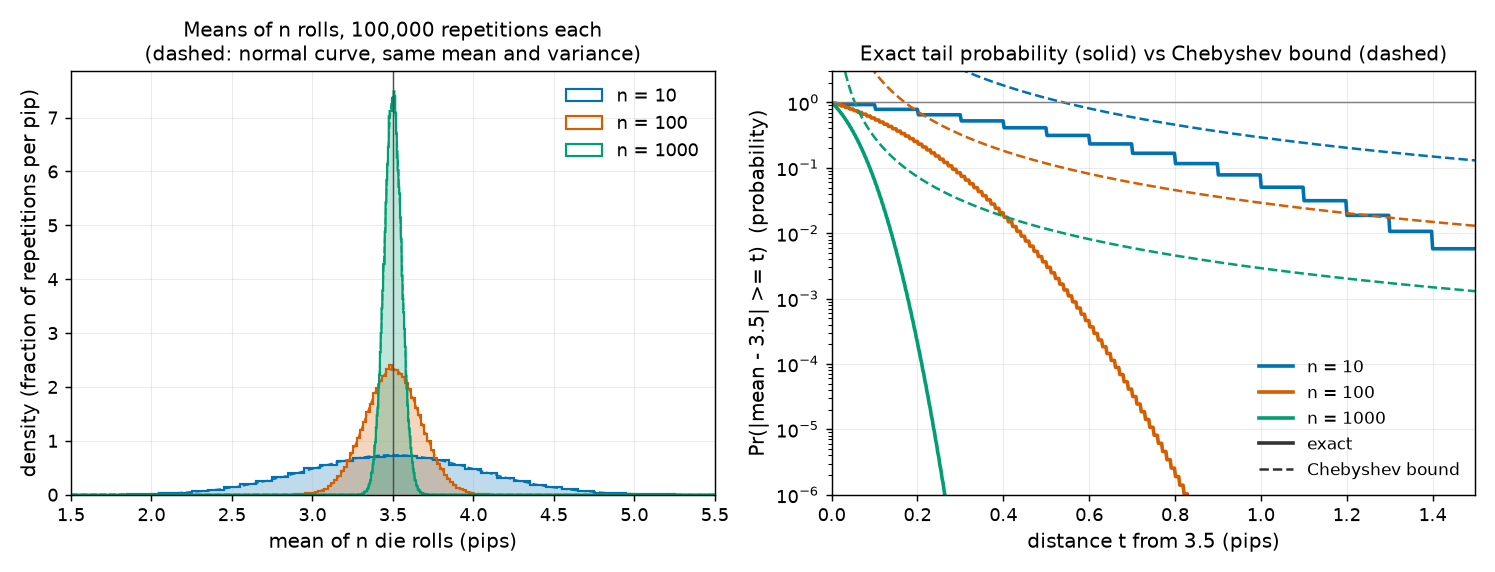
Left: the histograms narrow as \(n\) grows. That is the law of large numbers at work. The dashed bell curves are normal densities with the same mean and variance; they fit well. Right: the exact probability of missing 3.5 by at least \(t\) (solid) against Chebyshev's bound (dashed). Solid always stays below dashed of the same colour. For small \(t\) the dashed curve is above 1, where it says nothing.
Some individual numbers (simulated, then exact, then Chebyshev's bound):
- \(n=10\), miss by at least \(t=1\) pip: 0.07802, 0.07799, and the bound 0.2917. The bound holds with room to spare.
- \(n=10\), \(t=0.5\): exact 0.4099, while Chebyshev's bound is 1.1667. A "probability bound" above 1 is true but useless.
- Fix \(t=0.1\) and let \(n\) grow: exact probabilities 0.9273 (\(n=10\)), 0.5785 (\(n=100\)), 0.06541 (\(n=1000\)). Misses of a tenth of a pip go from near-certain to rare.
- A normal approximation for \(n=10\), \(t=1\) gives 0.06408, below the exact 0.07799. An approximation can err in either direction, so it is not a guarantee.
Markov's inequality bounds \(\Pr(\bar X_n\ge4.5)\) by 0.777778 for every \(n\). The exact values are 0.03899 for \(n=10\) and \(1.519\times10^{-9}\) for \(n=100\).
With versus without replacement¶
Population: the numbers 1 to 20 (\(N=20\)), with mean 10.5 and variance 33.25. Draw \(n=10\) of them, one million times with each scheme:
- With replacement: variance of the mean 3.3250 by formula (\(\sigma^2/n\)), 3.3248 simulated.
- Without replacement: 1.7500 by formula (\(\sigma^2/n\) times \(10/19=0.526316\)), 1.7495 simulated.
- Dependence, without replacement: the second draw is item 1 with probability 0.0500, but with probability 0.0000 when the first draw was item 1. With replacement the same conditional probability is 0.0492, the unconditional 0.05 up to simulation noise.
- Covariance of the first two draws: \(-1.7500\) by formula, \(-1.7727\) simulated (without replacement); 0.0325 simulated (with replacement, where the true value is 0).
At the paper's scale the difference is negligible:
SOURCE: nanoGPT prepare.py split The training set has \(m=8{,}009{,}762\) documents. The paper does not state this number (erratum E32).
PAPER §6.1, p. 7 The subsample has \(n=10{,}000\) documents.
MY EXPLANATION So the correction factor \((m-n)/(m-1)\) is 0.998752. Sampling with or without replacement makes almost no difference to the variance of the subsample mean.
Fixed versus random, run for real¶
The statement \(S\) was "\(|\bar X_{10}-3.5|<1\)", guaranteed to hold with probability at least 0.708333. One dataset (rolls 1, 1, 3, 6, 2, 2, 2, 4, 2, 4; mean 2.7) made it true. Among the first 20 of the 100,000 simulated datasets, one made it false (mean 4.7). Over all of them, \(S\) failed in a fraction 0.07802, within the guaranteed 0.29167.
The poll¶
For a poll of 1,000 voters the answers are 0 or 1, with variance at most 0.25. The usual 95 % margin of error, from the normal approximation, is 0.0310 (3.1 percentage points). Chebyshev's inequality with \(\delta=0.05\) guarantees a margin of 0.0707 (7.1 percentage points). The pollster's familiar number is an estimate; the guarantee costs more than twice as much.
Going deeper¶
Everything in this section is MY EXPLANATION.
The proofs sit next to the statements they prove, in collapsible blocks:
- consequences of the axioms (complement rule, monotonicity);
- expectation of a function, linearity and monotonicity of expectation;
- the variance formulas and the die's variance;
- the product rule for independent variables, covariance, the variance of a sum, and an uncorrelated-but-dependent example;
- the law of total probability and the tower rule;
- the normal density's total area, mean and variance;
- mean and variance of the sample mean;
- sampling without replacement: the negative covariance and the finite-population correction;
- Markov's inequality, Chebyshev's inequality, and the weak law of large numbers.
Two more topics follow.
Going deeper: what changes for continuous random variables
Sums over values become integrals against a density, and \(\Pr(X=x)=0\) for every single value \(x\). The definitions of independence, conditional expectation and variance carry over with integrals in place of sums. The proofs of linearity, Markov's inequality, Chebyshev's inequality and the law of large numbers go through unchanged, because they use only linearity and monotonicity of expectation.
For the paper, discrete theory is enough. A document is a finite string over a finite alphabet, so there are countably many possible documents and the document distribution is discrete. A loss computed from a document by a fixed model is then a discrete random variable too: it takes at most countably many values, even though those values are real numbers.
Going deeper: the observed dataset has probability 0 or 1
The claim "after seeing the data, \(S\) is either true or false" can be written with conditional probability. Let the data be the random object \(X\) and suppose we observed \(X=x\) (with \(\Pr(X=x)>0\)). Whether \(S\) holds is a function of the data, so the event "\(S\) holds and \(X=x\)" is either the whole event \(\{X=x\}\) (if \(S(x)\) is true) or empty (if not). Hence
The guarantee \(\Pr(S\text{ holds})\ge1-\delta\) is the average of these zeros and ones over the random data, by the law of total probability. A different framework (Bayesian statistics) does assign probabilities to unknown fixed quantities, by treating them as random. The paper's bounds are not statements of that kind.
Common misconceptions¶
- Misconception: "After computing a bound that holds with probability 0.95, there is a 95 % chance that it is true for my data." — Actually: the 95 % describes the procedure over repeated data collection. For your particular data the bound is either true or false (see "the observed dataset has probability 0 or 1" above).
- Misconception: "Documents that look alike, or come from the same website, cannot be independent." — Actually: independence is a property of how the documents are drawn, not of their content. The paper makes the same point in its §4.2 note (p. 5).
- Misconception: "Draws without replacement are i.i.d., because each draw is uniform." — Actually: each draw is uniform (identically distributed), but the draws are dependent. In the script, \(\Pr(D_2=1\mid D_1=1)=0.0000\) while \(\Pr(D_2=1)=0.0500\). This is the confusion behind erratum E05.
- Misconception: "Linearity of expectation needs independence." — Actually: it never does. What needs independence (or at least zero covariance) is the addition of variances and the product rule \(\mathbb E[XY]=\mathbb E[X]\,\mathbb E[Y]\).
- Misconception: "Markov's and Chebyshev's inequalities tell you roughly how likely a deviation is." — Actually: they are upper bounds and can be very loose: 0.2917 against the exact 0.07799, or 0.777778 against 0.03899 in the worked example. They can even exceed 1, which says nothing.
- Misconception: "By the law of large numbers, a run of high rolls will be balanced by low rolls later." — Actually: future rolls are independent of past ones. An early excess is diluted by many later rolls, not cancelled by opposite ones.
- Misconception: "The normal approximation (\(\pm1.96\) standard deviations) gives a guarantee." — Actually: it is an approximation. For 10 die rolls it gives 0.06408 where the exact probability is 0.07799, an underestimate. The paper's bounds must hold exactly at its actual sample size, so it uses inequalities.
Self-test¶
Q1. You roll a fair die \(n=100\) times. Use Chebyshev's inequality to bound the probability that the mean misses 3.5 by at least 0.5 pips. Then compare with the exact probability in the script output. Is the bound correct? Is it accurate?
Answer
The variance of one roll is \(\sigma^2=35/12\approx2.9167\) pips². Chebyshev gives \(\Pr(|\bar X_{100}-3.5|\ge0.5)\le\frac{\sigma^2}{n t^2}=\frac{2.9167}{100\times0.25}\approx0.1167\) (the script prints 0.1167). The exact probability is 0.003646 (simulated: 0.00353). The bound is correct: the truth is below it. It is not accurate: it is more than ten times the true value, because Chebyshev uses only the variance.
Q2. A paper states: "With probability at least 0.95, \(R(h)\le\hat R(h)+0.01\)." Here \(\hat R(h)\) is a model's average error on its training data and \(R(h)\) its average error on all possible data. What is random in this sentence, and what is fixed? After you have trained the model and computed \(\hat R(h)\), may you say "there is a 95 % chance that \(R(h)\le\hat R(h)+0.01\)"?
Answer
Random: the training data, and everything computed from them: \(\hat R(h)\) and the trained model \(h\) itself. Fixed: the source the data come from, the confidence level 0.95 (so \(\delta=0.05\)), the margin 0.01, and the number of training examples. For any one model chosen in advance, \(R(h)\) is a fixed number; for the trained model it is a fixed function evaluated at a random model.
No. The 0.95 is a property of the procedure: if the whole data collection and training were repeated many times, the inequality would fail in at most 5 % of the repetitions. For the data you actually have, the inequality is either true or false. You do not know which, because \(R(h)\) is unknown. What you may say is: "this bound was produced by a method that is wrong at most 5 % of the time".
Q3. The population is the numbers 1 to 20 (variance 33.25). (a) You draw \(n=20\) of them with replacement. What is the variance of the sample mean? (b) Same, without replacement. (c) Which scheme gives i.i.d. draws? (d) The paper draws a subsample of \(n=10{,}000\) from \(m=8{,}009{,}762\) documents. Would the choice of scheme change the variance of the subsample mean noticeably?
Answer
(a) \(\sigma^2/n=33.25/20=1.6625\). Some numbers appear twice and others not at all, so the mean varies.
(b) The correction factor is \((N-n)/(N-1)=(20-20)/19=0\), so the variance is 0. Drawing 20 of 20 items without replacement always gives the whole population, whose mean is exactly 10.5.
(c) Only sampling with replacement. Without replacement, each draw is uniform on its own, but the draws are dependent (a drawn item cannot reappear).
(d) No. The factor \((m-n)/(m-1)\) is 0.998752, with \(m=8{,}009{,}762\) taken from nanoGPT's data split SOURCE: nanoGPT prepare.py because the paper does not state it (erratum E32). The variance would shrink by only about a tenth of a percent.
Code for this chapter¶
Run it from the project root:
.venv/Scripts/python explainer/code/ch01_probability.py
Source: ch01_probability.py
"""Chapter 1 demo: the probability toolkit, checked by simulation.

Claims illustrated (all [MY EXPLANATION]; no paper numbers are reproduced here):
  [1] A fair die has E[X] = 3.5 pips and Var[X] = 35/12 squared pips (exact fractions).
  [2] The mean of n i.i.d. die rolls has variance sigma^2/n (n = 10, 100, 1000; 100,000 repetitions each).
  [3] Tail probabilities Pr(|mean - 3.5| >= t) shrink with n (law of large numbers) and never exceed
      Chebyshev's bound sigma^2/(n t^2). Exact values come from convolving the die's distribution n times.
  [4] Markov's bound Pr(mean >= 4.5) <= 3.5/4.5 holds (and is very loose).
  [5] Population {1,...,20}, n = 10 draws: Var(mean) = sigma^2/n with replacement and
      sigma^2/n * (N-n)/(N-1) without replacement; draws without replacement are dependent.
  [6] "Fixed vs random": one dataset makes a statement true or false; the probability describes the procedure.
  [7] Preview of Chapter 9: deviation t guaranteed with probability >= 1 - delta, Chebyshev vs Hoeffding.
  [8] The polling analogy: 95% margin of error for 1,000 voters, normal estimate vs Chebyshev guarantee.
Paper-related constants (m, n, delta) come from pacbound.py; m and delta are [SOURCE], not stated in the paper.

Writes outputs/ch01_probability.txt and docs/assets/fig/ch01_dice_means.png. Runtime: a few seconds.
"""
import math
import sys
from fractions import Fraction
from pathlib import Path

import numpy as np
from scipy.stats import norm

HERE = Path(__file__).resolve().parent
sys.path.insert(0, str(HERE))
import pacbound  # noqa: E402

import matplotlib  # noqa: E402
matplotlib.use("Agg")
import matplotlib.pyplot as plt  # noqa: E402
from matplotlib.lines import Line2D  # noqa: E402

OUT_TXT = HERE / "outputs" / "ch01_probability.txt"
OUT_FIG = HERE.parent / "docs" / "assets" / "fig" / "ch01_dice_means.png"
OUT_TXT.parent.mkdir(parents=True, exist_ok=True)
OUT_FIG.parent.mkdir(parents=True, exist_ok=True)

REPS = 100_000
NS = [10, 100, 1000]
TS = [0.1, 0.25, 0.5, 1.0]
COLORS = {10: "#0072B2", 100: "#D55E00", 1000: "#009E73"}
rng = np.random.default_rng(0)
lines = []


def out(s=""):
    lines.append(s)


# ---------------------------------------------------------------- [1] one die
faces = [Fraction(k) for k in range(1, 7)]
E1 = sum(faces) / 6
E2 = sum(f * f for f in faces) / 6
VAR1 = E2 - E1 * E1
assert E1 == Fraction(7, 2) and VAR1 == Fraction(35, 12)
MU, SIG2 = float(E1), float(VAR1)
SIG = math.sqrt(SIG2)
out("Chapter 1 demo (seed 0; 100,000 repetitions unless stated)")
out(f"[1] One fair die: E[X] = {E1} = {MU} pips; E[X^2] = {E2}; "
    f"Var[X] = {VAR1} = {SIG2:.6f} pips^2; sd = {SIG:.6f} pips")
# uncorrelated but dependent: U uniform on {-1, 0, 1}, W = U^2 (exact fractions)
third = Fraction(1, 3)
cov_uw = sum(third * u * u * u for u in (-1, 0, 1)) - sum(third * u for u in (-1, 0, 1)) * sum(
    third * u * u for u in (-1, 0, 1))
p_joint, p_prod = third, third * third        # Pr(U=0, W=0) = Pr(U=0) ; Pr(U=0) Pr(W=0)
assert cov_uw == 0 and p_joint != p_prod
p_even = Fraction(3, 6)
p_six_given_even = Fraction(1, 6) / p_even
out(f"    Pr(even) = {p_even}; Pr(roll = 6 | even) = (1/6)/(1/2) = {p_six_given_even}; "
    f"two dice: E[X1+X2] = E[E[X1+X2 | X1]] = E[X1 + 3.5] = {E1 + E1}")
out(f"    uncorrelated yet dependent: U uniform on {{-1,0,1}}, W = U^2: Cov(U,W) = {cov_uw}, "
    f"Pr(U=0,W=0) = {p_joint} but Pr(U=0)Pr(W=0) = {p_prod}")


# ------------------------------------------------- exact distribution of sums
def sum_pmf(n):
    """pmf of S = sum of n fair dice; index s - n holds Pr(S = s), s = n..6n."""
    p = np.ones(6) / 6.0
    pmf = np.array([1.0])
    for _ in range(n):
        pmf = np.convolve(pmf, p)
    return pmf


def exact_two_sided(pmf, n, t):
    """Pr(|S/n - 3.5| >= t) computed exactly from the pmf of S."""
    s = np.arange(n, 6 * n + 1)
    return float(pmf[np.abs(2 * s - 7 * n) >= 2 * t * n - 1e-9].sum())


def exact_upper(pmf, n, a):
    """Pr(S/n >= a)."""
    s = np.arange(n, 6 * n + 1)
    return float(pmf[s >= a * n - 1e-9].sum())


# ------------------------------------------------------ [2] simulate n rolls
sums = {}
for n in NS:
    chunks = []
    for _ in range(10):  # 10 chunks of 10,000 repetitions keeps memory small
        rolls = rng.integers(1, 7, size=(REPS // 10, n), dtype=np.int8)
        chunks.append(rolls.sum(axis=1, dtype=np.int64))
    sums[n] = np.concatenate(chunks)
pmfs = {n: sum_pmf(n) for n in NS}

out("[2] Mean of n rolls: variance formula sigma^2/n vs simulation (pips^2), sd in pips")
out("      n   Var formula   Var simulated   sd formula")
for n in NS:
    means = sums[n] / n
    vf, vs = SIG2 / n, float(np.var(means))
    assert abs(vs / vf - 1) < 0.02
    out(f"  {n:5d}   {vf:11.6f}   {vs:13.6f}   {math.sqrt(vf):10.6f}")

# ------------------------------------------------- [3] tails vs Chebyshev
out("[3] Pr(|mean - 3.5| >= t): simulated, exact, Chebyshev bound sigma^2/(n t^2)")
out("      n     t (pips)   simulated   exact        Chebyshev")
for n in NS:
    for t in TS:
        sim = float(np.mean(np.abs(2 * sums[n] - 7 * n) >= 2 * t * n - 1e-9))
        ex = exact_two_sided(pmfs[n], n, t)
        cheb = SIG2 / (n * t * t)
        se = math.sqrt(max(ex * (1 - ex), 1e-12) / REPS)
        assert abs(sim - ex) < 5 * se + 2e-5          # simulation agrees with exact
        assert ex <= cheb                              # Chebyshev holds
        note = "  (>1: says nothing)" if cheb > 1 else ""
        out(f"  {n:5d}   {t:6.2f}     {sim:9.5f}   {ex:.3e}    {cheb:8.4f}{note}")
z = 1.0 / math.sqrt(SIG2 / 10)
normal_approx = 2 * norm.sf(z)
out(f"    normal approximation for n=10, t=1: 2*(1-Phi({z:.4f})) = {normal_approx:.5f} "
    f"(exact {exact_two_sided(pmfs[10], 10, 1.0):.5f}) -- an estimate, not a bound")
out(f"    standard normal: Pr(|Z| >= 1.96) = {2 * norm.sf(1.96):.5f}")

# ------------------------------------------------------------ [4] Markov
out(f"[4] Markov: Pr(mean >= 4.5) <= E[mean]/4.5 = 3.5/4.5 = {3.5 / 4.5:.6f} for every n")
for n in NS:
    sim = float(np.mean(2 * sums[n] >= 9 * n))
    ex = exact_upper(pmfs[n], n, 4.5)
    assert ex <= 3.5 / 4.5
    out(f"    n = {n:4d}: simulated {sim:.5f}, exact {ex:.3e}")

# ------------------------------------------- [5] with vs without replacement
N, n_pop = 20, 10
pop = np.arange(1, N + 1)
mu_p, s2_p = float(pop.mean()), float(pop.var())
assert s2_p == (N * N - 1) / 12
REPS_POP = 1_000_000          # more repetitions here so the covariance estimates are precise
d_with = np.empty((REPS_POP, n_pop), dtype=np.int64)
d_wo = np.empty((REPS_POP, n_pop), dtype=np.int64)
for c in range(10):
    sl = slice(c * REPS_POP // 10, (c + 1) * REPS_POP // 10)
    k = REPS_POP // 10
    d_with[sl] = pop[rng.integers(0, N, size=(k, n_pop))]                     # put back after each draw
    d_wo[sl] = pop[np.argsort(rng.random((k, N)), axis=1)[:, :n_pop]]        # random order, keep first n
v_with_f = s2_p / n_pop
fpc = (N - n_pop) / (N - 1)
v_wo_f = v_with_f * fpc
v_with_s = float(np.var(d_with.mean(axis=1)))
v_wo_s = float(np.var(d_wo.mean(axis=1)))
assert abs(v_with_s / v_with_f - 1) < 0.01 and abs(v_wo_s / v_wo_f - 1) < 0.01
out(f"[5] Population {{1..{N}}}: mu = {mu_p}, sigma^2 = {s2_p} (= (N^2-1)/12); n = {n_pop} draws, "
    f"{REPS_POP:,} repetitions")
out(f"    with replacement   : Var(mean) formula sigma^2/n = {v_with_f:.4f}, simulated {v_with_s:.4f}")
out(f"    without replacement: formula sigma^2/n*(N-n)/(N-1) = {v_wo_f:.4f}, simulated {v_wo_s:.4f}"
    f"  (factor {N - n_pop}/{N - 1} = {fpc:.6f})")
p2 = float(np.mean(d_wo[:, 1] == 1))
first1 = d_wo[:, 0] == 1
p2_given = float(np.mean(d_wo[first1, 1] == 1))
p2_given_with = float(np.mean(d_with[d_with[:, 0] == 1, 1] == 1))
assert p2_given == 0.0
cov_f = -s2_p / (N - 1)
cov_s = float(np.cov(d_wo[:, 0], d_wo[:, 1])[0, 1])
cov_with_s = float(np.cov(d_with[:, 0], d_with[:, 1])[0, 1])
assert abs(cov_s - cov_f) < 0.15 and abs(cov_with_s) < 0.15 and abs(p2 - 1 / N) < 0.002
out(f"    without repl.: Pr(D2=1) = {p2:.4f} (formula 1/{N} = {1 / N:.4f}), Pr(D2=1 | D1=1) = {p2_given:.4f}")
out(f"    with repl.   : Pr(D2=1 | D1=1) = {p2_given_with:.4f}  -> only the with-replacement draws are independent")
out(f"    Cov(D1,D2): without repl. formula -sigma^2/(N-1) = {cov_f:.4f}, simulated {cov_s:.4f};"
    f" with repl. simulated {cov_with_s:.4f}")
out(f"    n = N = {N}: Var(mean) with repl. = sigma^2/N = {s2_p / N:.4f}; without repl. = "
    f"{s2_p / N * (N - N) / (N - 1):.4f} (every draw of the whole population has mean {mu_p})")
fpc_paper = (pacbound.M_DOCS - pacbound.N_SUB) / (pacbound.M_DOCS - 1)
out(f"    paper scale: (m-n)/(m-1) with m = {pacbound.M_DOCS:,} [SOURCE nanoGPT], n = {pacbound.N_SUB:,}: "
    f"{fpc_paper:.6f}")

# ---------------------------------------------------- [6] fixed vs random
out("[6] Fixed vs random. Statement S: |mean of 10 rolls - 3.5| < 1. Chebyshev: Pr(S false) <= "
    f"{SIG2 / 10:.6f}, so S holds w.p. >= {1 - SIG2 / 10:.6f}")
one = rng.integers(1, 7, size=10)
m1 = one.mean()
out(f"    one dataset: rolls {' '.join(map(str, one))} -> mean {m1:.1f} -> S is "
    f"{'TRUE' if abs(m1 - 3.5) < 1 else 'FALSE'} (a fact about this dataset, not a probability)")
means10 = sums[10] / 10
first = means10[:20]
out("    the first 20 of the 100,000 datasets from [2] (n=10), mean and S:")
for row in (first[:10], first[10:]):
    out("     " + "  ".join(f"{m:.1f}{'T' if abs(m - 3.5) < 1 else 'F'}" for m in row))
fail = float(np.mean(np.abs(sums[10] - 35) >= 10))
out(f"    S false in {fail:.5f} of the 100,000 datasets (exact {exact_two_sided(pmfs[10], 10, 1.0):.5f}; "
    f"guaranteed <= {SIG2 / 10:.5f})")

# ----------------------------------------- [7] Chebyshev vs Hoeffding preview
out(f"[7] Deviation t (pips) guaranteed w.p. >= 1-delta for the mean of n = 100 rolls (range width 5 pips)")
out("    delta       Chebyshev sigma/sqrt(n delta)   Hoeffding 5*sqrt(ln(2/delta)/(2n))  [Chapter 9]")
for d in [pacbound.DELTA, 1e-6, 1e-30]:
    t_cheb = SIG / math.sqrt(100 * d)
    t_hoef = pacbound.hoeffding_t(100, 5.0, math.log(2.0 / d))
    out(f"    {d:8.0e}    {t_cheb:20.4g}             {t_hoef:12.4f}")
t05 = SIG / math.sqrt(100 * pacbound.DELTA)
fail100 = float(np.mean(np.abs(2 * sums[100] - 700) >= 2 * 100 * t05))
out(f"    delta = {pacbound.DELTA}: Chebyshev t = {t05:.4f}; datasets (n=100) with |mean-3.5| >= t: "
    f"simulated {fail100:.5f}, exact {exact_two_sided(pmfs[100], 100, t05):.2e}")

# --------------------------------------------- [8] the polling analogy in numbers
n_poll, p_worst = 1000, 0.5                   # answers are 0/1; variance p(1-p) is largest at p = 0.5
var_ans = p_worst * (1 - p_worst)
margin_normal = 1.96 * math.sqrt(var_ans / n_poll)
margin_cheb = math.sqrt(var_ans / (n_poll * pacbound.DELTA))
out(f"[8] Poll of {n_poll:,} voters (0/1 answers, worst case variance {var_ans}): 95% margin of error")
out(f"    normal approximation 1.96*sqrt(0.25/n) = {margin_normal:.4f} "
    f"({100 * margin_normal:.1f} percentage points, an estimate)")
out(f"    Chebyshev guarantee sqrt(0.25/(n*0.05)) = {margin_cheb:.4f} "
    f"({100 * margin_cheb:.1f} percentage points, a guarantee)")

# ------------------------------------------------------------------ figure
fig, (ax1, ax2) = plt.subplots(1, 2, figsize=(11.5, 4.4))
grid = np.linspace(1.5, 5.5, 2001)
for n, width in [(10, 0.1), (100, 0.02), (1000, 0.005)]:
    means = sums[n] / n
    lo = (n - 0.5) / n
    edges = np.arange(lo, 6.0 + width, width)        # bin width = whole number of lattice steps 1/n
    ax1.hist(means, bins=edges, density=True, histtype="stepfilled", alpha=0.25, color=COLORS[n])
    ax1.hist(means, bins=edges, density=True, histtype="step", lw=1.2, color=COLORS[n],
             label=f"n = {n}")
    sd = math.sqrt(SIG2 / n)
    ax1.plot(grid, norm.pdf(grid, MU, sd), ls="--", lw=1.0, color=COLORS[n])
ax1.axvline(MU, color="0.3", lw=0.8)
ax1.set_xlim(1.5, 5.5)
ax1.set_xlabel("mean of n die rolls (pips)", fontsize=11)
ax1.set_ylabel("density (fraction of repetitions per pip)", fontsize=11)
ax1.set_title("Means of n rolls, 100,000 repetitions each\n(dashed: normal curve, same mean and variance)",
              fontsize=11)
ax1.legend(fontsize=10, frameon=False)

tgrid = np.linspace(0.005, 1.5, 600)
for n in NS:
    ex = [exact_two_sided(pmfs[n], n, t) for t in tgrid]
    ax2.plot(tgrid, np.maximum(ex, 1e-12), color=COLORS[n], lw=2)
    ax2.plot(tgrid, np.minimum(SIG2 / (n * tgrid ** 2), 10), color=COLORS[n], lw=1.4, ls="--")
ax2.axhline(1.0, color="0.5", lw=0.8)
ax2.set_yscale("log")
ax2.set_ylim(1e-6, 3)
ax2.set_xlim(0, 1.5)
ax2.set_xlabel("distance t from 3.5 (pips)", fontsize=11)
ax2.set_ylabel("Pr(|mean - 3.5| >= t)  (probability)", fontsize=11)
ax2.set_title("Exact tail probability (solid) vs Chebyshev bound (dashed)", fontsize=11)
handles = [Line2D([], [], color=COLORS[n], lw=2, label=f"n = {n}") for n in NS]
handles += [Line2D([], [], color="0.2", lw=2, label="exact"),
            Line2D([], [], color="0.2", lw=1.4, ls="--", label="Chebyshev bound")]
ax2.legend(handles=handles, fontsize=9.5, frameon=False, loc="lower right")
for ax in (ax1, ax2):
    ax.grid(alpha=0.25, lw=0.6)
    ax.tick_params(labelsize=10)
fig.tight_layout()
fig.savefig(OUT_FIG, dpi=130)
out(f"figure: docs/assets/fig/{OUT_FIG.name}")

text = "\n".join(lines) + "\n"
print(text, end="")
OUT_TXT.write_text(text, encoding="utf-8")
Output:
Chapter 1 demo (seed 0; 100,000 repetitions unless stated)
[1] One fair die: E[X] = 7/2 = 3.5 pips; E[X^2] = 91/6; Var[X] = 35/12 = 2.916667 pips^2; sd = 1.707825 pips
    Pr(even) = 1/2; Pr(roll = 6 | even) = (1/6)/(1/2) = 1/3; two dice: E[X1+X2] = E[E[X1+X2 | X1]] = E[X1 + 3.5] = 7
    uncorrelated yet dependent: U uniform on {-1,0,1}, W = U^2: Cov(U,W) = 0, Pr(U=0,W=0) = 1/3 but Pr(U=0)Pr(W=0) = 1/9
[2] Mean of n rolls: variance formula sigma^2/n vs simulation (pips^2), sd in pips
      n   Var formula   Var simulated   sd formula
     10      0.291667        0.292320     0.540062
    100      0.029167        0.028976     0.170783
   1000      0.002917        0.002922     0.054006
[3] Pr(|mean - 3.5| >= t): simulated, exact, Chebyshev bound sigma^2/(n t^2)
      n     t (pips)   simulated   exact        Chebyshev
     10     0.10       0.92820   9.273e-01     29.1667  (>1: says nothing)
     10     0.25       0.65115   6.479e-01      4.6667  (>1: says nothing)
     10     0.50       0.41134   4.099e-01      1.1667  (>1: says nothing)
     10     1.00       0.07802   7.799e-02      0.2917
    100     0.10       0.57584   5.785e-01      2.9167  (>1: says nothing)
    100     0.25       0.15010   1.516e-01      0.4667
    100     0.50       0.00353   3.646e-03      0.1167
    100     1.00       0.00000   3.038e-09      0.0292
   1000     0.10       0.06674   6.541e-02      0.2917
   1000     0.25       0.00000   3.757e-06      0.0467
   1000     0.50       0.00000   1.541e-20      0.0117
   1000     1.00       0.00000   2.224e-79      0.0029
    normal approximation for n=10, t=1: 2*(1-Phi(1.8516)) = 0.06408 (exact 0.07799) -- an estimate, not a bound
    standard normal: Pr(|Z| >= 1.96) = 0.05000
[4] Markov: Pr(mean >= 4.5) <= E[mean]/4.5 = 3.5/4.5 = 0.777778 for every n
    n =   10: simulated 0.03933, exact 3.899e-02
    n =  100: simulated 0.00000, exact 1.519e-09
    n = 1000: simulated 0.00000, exact 1.112e-79
[5] Population {1..20}: mu = 10.5, sigma^2 = 33.25 (= (N^2-1)/12); n = 10 draws, 1,000,000 repetitions
    with replacement   : Var(mean) formula sigma^2/n = 3.3250, simulated 3.3248
    without replacement: formula sigma^2/n*(N-n)/(N-1) = 1.7500, simulated 1.7495  (factor 10/19 = 0.526316)
    without repl.: Pr(D2=1) = 0.0500 (formula 1/20 = 0.0500), Pr(D2=1 | D1=1) = 0.0000
    with repl.   : Pr(D2=1 | D1=1) = 0.0492  -> only the with-replacement draws are independent
    Cov(D1,D2): without repl. formula -sigma^2/(N-1) = -1.7500, simulated -1.7727; with repl. simulated 0.0325
    n = N = 20: Var(mean) with repl. = sigma^2/N = 1.6625; without repl. = 0.0000 (every draw of the whole population has mean 10.5)
    paper scale: (m-n)/(m-1) with m = 8,009,762 [SOURCE nanoGPT], n = 10,000: 0.998752
[6] Fixed vs random. Statement S: |mean of 10 rolls - 3.5| < 1. Chebyshev: Pr(S false) <= 0.291667, so S holds w.p. >= 0.708333
    one dataset: rolls 1 1 3 6 2 2 2 4 2 4 -> mean 2.7 -> S is TRUE (a fact about this dataset, not a probability)
    the first 20 of the 100,000 datasets from [2] (n=10), mean and S:
     4.1T  4.2T  2.6T  2.8T  3.3T  3.7T  4.1T  3.8T  4.0T  4.7F
     3.6T  3.9T  3.4T  3.4T  3.3T  2.7T  3.0T  3.4T  3.4T  4.0T
    S false in 0.07802 of the 100,000 datasets (exact 0.07799; guaranteed <= 0.29167)
[7] Deviation t (pips) guaranteed w.p. >= 1-delta for the mean of n = 100 rolls (range width 5 pips)
    delta       Chebyshev sigma/sqrt(n delta)   Hoeffding 5*sqrt(ln(2/delta)/(2n))  [Chapter 9]
       5e-02                  0.7638                   0.6791
       1e-06                   170.8                   1.3467
       1e-30               1.708e+14                   2.9532
    delta = 0.05: Chebyshev t = 0.7638; datasets (n=100) with |mean-3.5| >= t: simulated 0.00000, exact 6.12e-06
[8] Poll of 1,000 voters (0/1 answers, worst case variance 0.25): 95% margin of error
    normal approximation 1.96*sqrt(0.25/n) = 0.0310 (3.1 percentage points, an estimate)
    Chebyshev guarantee sqrt(0.25/(n*0.05)) = 0.0707 (7.1 percentage points, a guarantee)
figure: docs/assets/fig/ch01_dice_means.png