07. Training neural networks¶
Where this fits
Prerequisites: Chapter 2 (model, parameter, hypothesis, loss, empirical risk, training, overfitting) and Chapter 8 (vector, matrix, transpose, matrix–vector product, dot product, norm, orthonormal columns, Cauchy–Schwarz). It also uses neural network, layer, weight matrix and bias from Chapter 5; a reminder is given where they first appear. Used later by: Chapter 18 (random subspace training), Chapter 19 (LoRA), Chapter 20 (SubLoRA), Chapter 21 (quantization-aware training) and Chapter 28 (mini replication). Purpose: explain how the paper's models are actually trained — gradient descent and its variants, how a gradient passes through the change of variables \(\theta=\theta_0+Pw\), and why a random starting point costs only a seed.
The problem this chapter solves¶
MY EXPLANATION Chapter 2 described training as a procedure that takes the training set and returns one hypothesis \(\hat h\). It did not say how. For a model with three parameters you could try many combinations of values and keep the best. GPT-2 small has 123,689,472 parameters in nanoGPT's counting (script output [7]). Trying combinations is hopeless.
Neural networks are instead trained by improving their parameters a little at a time. At each step the training program asks one local question: "if I nudge each parameter slightly, does the loss go up or down, and how fast?" It then moves every parameter a small amount in the direction that lowers the loss. This chapter makes that precise.
PAPER §3, p. 4 The paper relies on this machinery in three places. First, in subspace training the weights are written \(\theta=\theta_0+Pw\), where \(\theta_0\) is a random initialization and \(P\) a fixed matrix, and only the short vector \(w\) is optimized "by backpropagating through the transformation".
PAPER §5, p. 6 Second, SubLoRA uses a nonlinear version, \(\theta=\theta_0+\mathrm{LoRA}(Pw)\). The authors call \(\theta_0\) merely a random initialization, and say that \(\theta_0\) and \(P\) are chosen ahead of time, so only \(w\) has to be stored.
PAPER App. E, p. 16 Third, the optimizer is AdamW with weight decay \(10^{-2}\) and \(\epsilon=10^{-6}\); batches of 8 sequences of 1,024 tokens are sampled with replacement; the learning rate is searched over \(\{2\times10^{-4},\,5\times10^{-3},\,5\times10^{-5}\}\).
MY EXPLANATION By the end of the chapter every phrase in those three paragraphs will have an exact meaning. We answer three questions. How does one training step work? How does the gradient reach \(w\) when the model is written as \(\theta=\theta_0+Pw\)? And why may the bound treat a random \(\theta_0\) with over a hundred million numbers as free?
Intuition (and where the analogy breaks)¶
Everything in this section is MY EXPLANATION.
A hiker stands on a hillside in thick fog. She wants to reach low ground. She cannot see the valley. She can only feel the slope of the ground under her feet.
Her strategy: feel which way the ground falls most steeply, take a step that way, and repeat. Each step is small, so the slope she felt is still roughly right while she takes it.
The mapping: her position is the list of parameter values. The height of the ground is the loss. The slope under her feet is the gradient. The length of her step is set by the learning rate.
Now chain the hiker to a straight trail that runs across the hillside. She can still walk downhill along the trail. But the lowest point of the trail may lie far above the valley floor. That is training through a reparameterization \(\theta=\theta_0+Pw\): only the points on the "trail" can be reached.
Where it breaks:
- Dimensions. The hiker has two directions to choose from. GPT-2 small has over a hundred million. Pictures in two dimensions are a guide, not a proof.
- Noisy slope. In practice the slope is not measured on all the training data. It is estimated from a small random handful of examples (a minibatch). That is like feeling the ground through a shaky stick: right on average, wrong in any single reading.
- No unique bottom, and no need for one. A neural network's loss landscape has many valleys. Training stops long before any exact bottom. For the paper's bound this does not matter: the bound is computed for whatever point training ends at.
- Step size is not natural. A hiker shortens her stride on steep ground. Gradient descent takes a step proportional to the slope, so on a steep wall a large step overshoots and lands higher on the opposite wall. In the worked example below, a learning rate of 0.11 makes the loss explode to 828 million.
Precise definition¶
Everything in this section is MY EXPLANATION unless tagged.
Notation. The parameters are a vector \(\theta=(\theta_1,\dots,\theta_D)\in\mathbb R^D\). The function we minimize is written \(\mathcal L(\theta)\) and called the training objective. Usually it is the empirical risk of Chapter 2, viewed as a function of the parameters:
Here \(X_1,\dots,X_m\) are the \(m\) training examples and \(\ell(\theta,X_j)\) is the loss, on example \(X_j\), of the hypothesis whose parameters are \(\theta\) (Chapter 2 writes it \(R(h,X_j)\)). Training produces a sequence of parameter vectors. We write the one after \(t\) steps as \(\theta^{(t)}\), with the step number in brackets above, so that \(\theta_k\) (below) still means "coordinate \(k\)". The starting point \(\theta^{(0)}\) is what the paper calls \(\theta_0\).
Derivative and partial derivative¶
The derivative of a function \(f\) of one number is its slope:
In words: move \(x\) by a tiny amount \(\varepsilon\), see how much \(f\) changes, divide by \(\varepsilon\). The practical meaning is the approximation \(f(x+\varepsilon)\approx f(x)+f'(x)\,\varepsilon\) for small \(\varepsilon\).
Example: \(f(x)=(x-3)^2\). Then \(\big(f(x+\varepsilon)-f(x)\big)/\varepsilon=\big((x-3+\varepsilon)^2-(x-3)^2\big)/\varepsilon =2(x-3)+\varepsilon\), which tends to \(f'(x)=2(x-3)\). At \(x=0\) the slope is \(-6\): moving right lowers \(f\).
A partial derivative is the same idea for a function of several numbers: change one of them, hold all others fixed. It is written \(\partial\mathcal L/\partial\theta_k\). For the function used throughout this chapter,
The gradient¶
The gradient is the vector of all partial derivatives:
The symbol \(\nabla\) is read "nabla" or "grad". At \(\theta=(0,0)\) the example gives \(\nabla\mathcal L=(-6,20)\) (output [1]).
Two facts make the gradient useful. First, for a small change \(\Delta\) of the parameters,
where "\(\cdot\)" is the dot product of Chapter 8. Second, as a consequence, \(-\nabla\mathcal L\) points in the direction in which the loss falls fastest, and at a lowest point the gradient is the zero vector.
Going deeper: the gradient is the direction of steepest ascent
What "differentiable" means. \(\mathcal L\) is differentiable at \(\theta\) if there is a vector \(g\) such that
The remainder \(r\) shrinks faster than the step. Taking \(\Delta=\varepsilon e_k\) (move only coordinate \(k\)) and dividing by \(\varepsilon\) shows \(g_k=\partial\mathcal L/\partial\theta_k\), so \(g=\nabla\mathcal L(\theta)\). (Existence of all partial derivatives alone does not guarantee this; continuous partial derivatives do. That standard theorem is skipped. Every function in this chapter has them.)
Rate of change in a direction. Let \(u\) be a unit vector. Put \(\Delta=\varepsilon u\):
Steepest direction. By Cauchy–Schwarz (Chapter 8), \(-\lVert\nabla\mathcal L\rVert\le\nabla\mathcal L\cdot u\le\lVert\nabla\mathcal L\rVert\) for every unit \(u\), with equality on the right exactly when \(u=\nabla\mathcal L/\lVert\nabla\mathcal L\rVert\) and on the left exactly when \(u=-\nabla\mathcal L/\lVert\nabla\mathcal L\rVert\). So the gradient is the direction of fastest increase and its negative the direction of fastest decrease. The fastest rate is \(\lVert\nabla\mathcal L\rVert\).
Zero gradient at a minimum. If \(\nabla\mathcal L(\theta)\ne0\), the rate along \(-\nabla\mathcal L\) is \(-\lVert\nabla\mathcal L\rVert<0\), so a small enough step lowers \(\mathcal L\), and \(\theta\) was not a minimum. The converse fails: a zero gradient can also sit at a maximum or a saddle point.
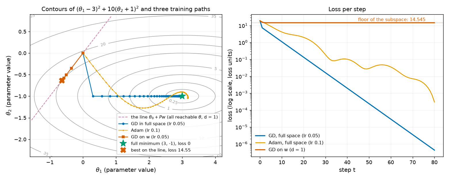
Perpendicular to contour lines. Along a contour line (a curve of constant loss) the rate of change is 0, so the gradient is perpendicular to the contour's direction. In the figure of the worked example, gradient descent leaves the start perpendicular to the ellipses.
Gradient descent and the learning rate¶
Gradient descent (GD) repeats one update:
Read it as: compute the slope at the current point, step against it, repeat. The positive number \(\eta\) ("eta") is the learning rate. It is chosen by hand. One update is one step (or iteration). Training stops after a fixed number of steps, or when the gradient is nearly zero.
The learning rate controls everything about speed and safety. Too small, and progress is slow. Too large, and each step overshoots the bottom of the valley. In the worked example, every learning rate of 0.1 or more fails (output [1]).
PAPER App. C, p. 15 Algorithm 1, line 12, writes this update for the subspace vector \(w\) and the quantization levels \(c\), using \(\rho\) for the learning rate: subtract \(\rho\) times the gradient of the loss.
Paper erratum E17: Algorithm 1 differentiates through rounding
PAPER App. C, p. 15 Line 12 updates \(w\) by its gradient while the loss is computed from the quantized weights, each of which is set to its nearest quantization level. MY EXPLANATION Rounding to the nearest level is a step function: its derivative is 0 almost everywhere, so a literal gradient would be zero and \(w\) would never move. Making line 12 work needs a straight-through estimator (pretend the rounding had derivative 1), which Chapter 21 explains. The algorithm does not mention it (erratum E17).
Going deeper: exactly when gradient descent converges on a bowl
Take the family of bowls \(\mathcal L(\theta)=\sum_{k=1}^{D}q_k(\theta_k-\theta^\star_k)^2\) with all \(q_k>0\). The worked example has \(q=(1,10)\) and \(\theta^\star=(3,-1)\).
The partial derivatives are \(2q_k(\theta_k-\theta^\star_k)\). Write \(e_k^{(t)}=\theta_k^{(t)}-\theta^\star_k\) for the error in coordinate \(k\). One GD step gives
Each coordinate is multiplied by its own shrink factor \(1-2\eta q_k\) every step, independently of the others. The loss is
It tends to 0 from every start exactly when \(|1-2\eta q_k|<1\) for every \(k\), i.e. \(0<\eta<1/q_k\) for every \(k\), i.e. \(\eta<1/\max_k q_k\). Here \(\max_k q_k=10\), so the condition is \(\eta<0.1\) (output [1]).
- At \(\eta=0.05\) the factors are \(0.90\) and \(0.00\) (output [1]). The second coordinate lands on \(-1\) in one step. After that the loss is \(1\cdot0.9^{2t}\cdot3^2=9\cdot0.81^t\), which first drops below \(10^{-6}\) at step 76.
- At \(\eta=0.1\) the second factor is \(-1\): the error flips sign forever, \(\theta_2\) bounces between 0 and \(-2\), and the loss stays at 10.
- At \(\eta=0.11\) the second factor is \(-1.2\): the error grows by 20 % per step and the loss reaches \(8.282\times10^{8}\) after 50 steps.
The slowest coordinate decides the speed. The best single \(\eta\) balances the two extreme factors, \(1-2\eta q_{\min}=-(1-2\eta q_{\max})\), giving \(\eta=1/(q_{\min}+q_{\max})\) and worst factor \((\kappa-1)/(\kappa+1)\) with \(\kappa=q_{\max}/q_{\min}\), the condition number. Long thin valleys (\(\kappa\) large) are slow for GD. That is one motivation for momentum and Adam below.
A general version for non-quadratic losses (the "descent lemma") needs the chain rule, so it is proved in the hub section Going deeper.
Stochastic gradient descent, minibatches and epochs¶
The gradient of an average is the average of the gradients (the derivative of a sum is the sum of the derivatives):
So one exact gradient costs one pass over all \(m\) training examples. [SOURCE: nanoGPT prepare.py] The
OpenWebText training split holds 9,035,582,198 tokens (output [8]). Paying that for every single step is out of the
question.
MY EXPLANATION A minibatch is a small random set \(\mathcal B\) of example indices. Its size \(|\mathcal B|\) is the batch size. The minibatch gradient replaces the average over all \(m\) examples by the average over the minibatch:
Stochastic gradient descent (SGD) is gradient descent with \(g\) in place of the exact gradient: \(\theta^{(t+1)}=\theta^{(t)}-\eta\,g^{(t)}\), with a fresh random minibatch at every step. "Stochastic" means random.
The minibatch gradient is right on average and its error shrinks as the batch grows. In the logistic-regression example below, the mean squared error of the minibatch gradient is 12.6040 with one example, 1.5742 with 8 and 0.1969 with 64, matching the formula \(\sigma^2/|\mathcal B|\) (output [5]).
An epoch is one pass through the whole training set. In the common scheme the examples are shuffled and cut into consecutive minibatches. With \(m=400\) examples and batch size 8 that is 50 steps per epoch.
PAPER App. E, p. 16 The paper's batches hold 8 sequences of 1,024 tokens, i.e. 8,192 tokens (output [8]), and
are sampled with replacement. MY EXPLANATION With replacement there are no clean epochs: some text is seen
twice before other text is seen once. For scale, one pass's worth of tokens in such batches would be 1,102,976 steps
(output [8]; token count from [SOURCE: nanoGPT prepare.py]). [SOURCE: authors' config
config_sublora_train.yaml] The released configuration also accumulates 40 minibatches before each update, i.e.
averages their gradients and then takes one step, which acts like a batch of 320 sequences (output [8]).
PAPER App. D, p. 16 The fine-tuning experiments, by contrast, are described in epochs: 5 of them.
Going deeper: the minibatch gradient is unbiased, and its noise falls like 1/|B|
What is random and what is fixed. The training set and the current \(\theta\) are fixed. The only randomness is the choice of minibatch indices \(i_1,\dots,i_b\) (\(b=|\mathcal B|\)), drawn independently and uniformly from \(\{1,\dots,m\}\) (with replacement, as in the paper).
Let \(G_c=\nabla\ell(\theta,X_{i_c})\), a random vector, and let \(\bar g=\frac1m\sum_j\nabla\ell(\theta,X_j)\) be the full gradient. Because \(i_c\) is uniform,
The minibatch gradient is unbiased. For its error, expand the squared norm of an average:
For \(c\ne c'\) the two factors are independent with mean zero, so the term is \(\mathbb E[G_c-\bar g]\cdot\mathbb E[G_{c'}-\bar g]=0\). The \(b\) terms with \(c=c'\) each equal \(\sigma^2=\frac1m\sum_j\lVert\nabla\ell(\theta,X_j)-\bar g\rVert^2\). Hence
This is Chapter 1's "variance of a sample mean is \(\sigma^2/n\)", applied to each coordinate and summed. Output [5] checks it at the starting point of the logistic regression: \(\sigma^2=12.6046\); simulated errors 12.6040, 1.5742, 0.1969 for \(b=1,8,64\) against formula values 12.6046, 1.5756, 0.1969; the average of 20,000 minibatch gradients misses the full gradient by only 0.67 %. Shuffled epochs sample without replacement; then the error is smaller by Chapter 1's factor \((m-b)/(m-1)\).
Momentum¶
Plain SGD zig-zags: noisy gradients point a little wrong at every step, and in long thin valleys even exact gradients point mostly across the valley rather than along it. Momentum steps along a running average of recent gradients instead of the latest one:
Here \(g^{(t)}\) is the gradient (or minibatch gradient) at step \(t\), and \(\beta\) is a number in \([0,1)\) that sets how long the memory is. Unrolling the first equation, \(u^{(t)}\) is a weighted average of all past gradients with weight \((1-\beta)\beta^{t-k}\) on step \(k\): recent gradients count most, old ones fade geometrically. Components that keep the same sign add up; components that flip sign cancel. Think of a heavy ball rolling down the landscape.
(Some libraries, e.g. PyTorch's SGD, write \(u^{(t)}=\beta u^{(t-1)}+g^{(t)}\) without the factor \(1-\beta\); that only rescales the learning rate.)
Adam, weight decay and AdamW¶
SOURCE: Kingma & Ba 2015, "Adam" Adam combines momentum with a separate step size for every parameter. It keeps two running averages, of the gradient and of the squared gradient (squares taken entry by entry):
MY EXPLANATION Symbol by symbol: \(u\) is the momentum average and \(v\) the average squared gradient, both starting at 0. \(\beta_1\) and \(\beta_2\) are their memory constants (common choices 0.9 and 0.999; \(\beta_1^{\,t}\) is \(\beta_1\) to the power \(t\)). The hats are bias corrections that undo the pull toward the starting value 0 in early steps. The division and square root act entry by entry. \(\epsilon\) is a small number that prevents division by zero. (The Adam paper calls \(u\) and \(v\) "\(m_t\)" and "\(v_t\)"; we rename the first because \(m\) is our number of training examples.)
The ratio \(\hat u/\sqrt{\hat v}\) is roughly "average gradient divided by its typical size". So each parameter moves by about \(\eta\) per step, whatever the scale of its gradient. Output [4]: on the worked example the first gradient is \((-6,20)\), yet Adam's first step with \(\eta=0.1\) moves to exactly \((0.1,-0.1)\), i.e. \(\eta\) times the sign of the gradient in each coordinate.
Weight decay shrinks every parameter slightly toward 0 at every step: \(\theta\leftarrow(1-\eta\lambda)\theta\), with a small constant \(\lambda\ge0\). It expresses a mild preference for small parameters. For plain GD it is the same as adding \(\tfrac{\lambda}{2}\lVert\theta\rVert^2\) to the loss; for Adam it is not (deeper block below).
[SOURCE: Loshchilov & Hutter 2017, arXiv 1711.05101; PyTorch torch.optim.AdamW] AdamW is Adam with
decoupled weight decay: first multiply the parameters by \((1-\eta\lambda)\), then take the Adam step computed from
the loss gradient alone. MY EXPLANATION Our hand-written Adam and AdamW agree with PyTorch's to \(4.4\times10^{-16}\)
and \(8.9\times10^{-16}\) over 300 steps (output [4]), so the equations above are exactly what the library runs.
PAPER App. E, p. 16 The paper uses AdamW with \(\lambda=10^{-2}\) and \(\epsilon=10^{-6}\). MY EXPLANATION With zero gradient, a weight is multiplied by \(1-\eta\lambda\) per step. For the three learning rates of the paper's grid the factors are 0.9999980, 0.9999500 and 0.9999995, and a weight would halve after 346,573, 13,863 and 1,386,294 steps respectively (output [4]).
MY ANALYSIS In subspace training the optimizer's parameters are \(w\), not \(\theta\). Weight decay therefore pulls \(w\) toward 0, which pulls \(\theta=\theta_0+Pw\) toward the random initialization \(\theta_0\) — not toward 0.
Paper erratum E48: the AdamW settings in App. E are incomplete
PAPER App. E, p. 16 The paper lists AdamW with weight decay \(10^{-2}\), epsilon \(10^{-6}\) "and no decay bias", without saying what "no decay bias" means.
[SOURCE: authors' code, projectors.py and config_sublora_train.yaml] In the code, a flag
no_decay_bias=True puts every parameter tensor with fewer than two dimensions into a group with weight decay 0.
In subspace and SubLoRA training the only trainable tensor is the one-dimensional vector \(w\). Under that reading
the stated weight decay would have no effect at all. The released configuration sets no_decay_bias: False, under
which \(w\) is decayed. The paper also leaves out \(\beta_1,\beta_2\) (config: 0.9, 0.999), the learning-rate schedule
(code default: linear warm-up for 2,000 steps, then cosine decay), gradient accumulation (config: 40 minibatches,
320 sequences per update), gradient clipping (code default: norm 1.0), the number of updates (config: at most
600,000) and the seeds (137 for \(\theta_0\) and \(P\), 1337 for batch sampling) — all printed in output [8].
MY ANALYSIS Impact: none on the validity of any bound, because the bound holds whatever procedure produced the final model (see "Hyperparameters" below). It affects only reproducibility.
Going deeper: Adam's bias correction and AdamW's decoupling, derived
Unrolling the average. Claim: \(u^{(t)}=(1-\beta_1)\sum_{k=1}^{t}\beta_1^{\,t-k}g^{(k)}\). For \(t=1\) it reads \(u^{(1)}=(1-\beta_1)g^{(1)}\), which is the update with \(u^{(0)}=0\). If it holds for \(t-1\), then
The weights do not sum to 1. Their sum is a geometric sum that telescopes:
The missing weight \(\beta_1^{\,t}\) sits on the starting value \(u^{(0)}=0\), which drags \(u^{(t)}\) toward 0 while \(t\) is small. Dividing by \(1-\beta_1^{\,t}\) makes the weights sum to 1: \(\hat u^{(t)}\) is a true weighted average. In particular, if every gradient equals the same \(g\), then \(\hat u^{(t)}=g\) exactly. The same argument applies to \(\hat v^{(t)}\).
The first step. At \(t=1\): \(\hat u^{(1)}=g^{(1)}\) and \(\hat v^{(1)}=(g^{(1)})^2\), so coordinate \(k\) moves by \(-\eta\,g_k/(|g_k|+\epsilon)\), which is \(-\eta\,\mathrm{sign}(g_k)\) up to the negligible \(\epsilon\). Output [4]: \(\theta^{(1)}=(0.100000,-0.100000)\), then \((0.199897,-0.199588)\) and \((0.299618,-0.298414)\). Without the correction the first step would be \((1-\beta_1)/\sqrt{1-\beta_2}\) times \(\eta\,\mathrm{sign}(g)\) instead.
Scale invariance. Multiply every gradient by a constant \(c>0\). Then \(\hat u\) scales by \(c\) and \(\sqrt{\hat v}\) by \(c\), so the step is unchanged (ignoring \(\epsilon\)). That is why Adam's steps have size about \(\eta\) per coordinate. It also explains the wobbly loss curve of Adam in the figure below: near the bottom the steps do not automatically shrink with the gradient. After 100 steps the loss is \(4.605\times10^{-4}\), after 300 steps \(2.274\times10^{-13}\) (output [4]).
Why "decoupled" matters. Adding the penalty \(\tfrac\lambda2\lVert\theta\rVert^2\) to the loss adds \(\lambda\theta\) to the gradient. In plain GD the update becomes \(\theta-\eta(g+\lambda\theta)=(1-\eta\lambda)\theta-\eta g\): exactly weight decay. In Adam the extra \(\lambda\theta_k\) passes through the division by \(\sqrt{\hat v_k}\), so coordinates with large past gradients are decayed weakly and coordinates with small gradients strongly. AdamW applies \((1-\eta\lambda)\) directly, so every coordinate decays at the same relative rate. In PyTorch's version the decay is multiplied by the current learning rate \(\eta\), which is why the per-step factors above are so close to 1.
The chain rule and backpropagation¶
A reminder from Chapter 5. A neural network is a model built from layers. A typical layer multiplies its input vector by a weight matrix, adds a bias vector, and then applies a simple nonlinear function to each entry. The output of one layer is the input of the next. So the loss is a long chain of simple functions applied one after another.
The chain rule of calculus says how slopes combine along such a chain. For one variable: if \(y=g(x)\) and \(z=f(y)\), then
Rates of change multiply. For many variables, if \(\mathcal L\) depends on \(\theta_1,\dots,\theta_D\) and each \(\theta_k\) depends on \(w_i\), then
Every path from \(w_i\) to \(\mathcal L\) contributes the product of the rates along it, and the contributions add.
Backpropagation applies the chain rule to a network starting at the loss and moving backward, layer by layer. At each layer it reuses the derivatives already computed for the layer above. The result is the gradient with respect to every parameter, at a cost of a small constant multiple of computing the loss once. Deep-learning libraries do this automatically ("autograd").
A finite-difference check estimates a partial derivative directly from its definition, \(\big(\mathcal L(\theta+he_k)-\mathcal L(\theta-he_k)\big)/(2h)\) for a small \(h\), where \(e_k\) is the vector with 1 in position \(k\) and 0 elsewhere. It costs two loss evaluations per parameter — for GPT-2 small, two for each of 123,689,472 parameters — so it is used only to test code. Output [3]: on a tiny network, backpropagation by hand agrees with PyTorch's autograd to \(0.0\) and with finite differences to \(1.0\times10^{-10}\).
Going deeper: the multivariable chain rule, and backpropagation worked by hand
The Jacobian. For a map \(f:\mathbb R^d\to\mathbb R^D\), \(w\mapsto\theta=f(w)\), the Jacobian matrix \(J_f(w)\in\mathbb R^{D\times d}\) has entries \((J_f)_{ki}=\partial\theta_k/\partial w_i\). Differentiability of \(f\) means \(f(w+\Delta)=f(w)+J_f(w)\Delta+r_1(\Delta)\) with \(\lVert r_1(\Delta)\rVert/\lVert\Delta\rVert\to0\).
Theorem (chain rule). If \(f\) is differentiable at \(w\) and \(\mathcal L\) at \(\theta=f(w)\), then \(\mathcal L\circ f\) is differentiable at \(w\) and
Entry \(i\) of the right side is \(\sum_k(\partial\theta_k/\partial w_i)(\partial\mathcal L/\partial\theta_k)\), the formula in the main text.
Proof. Put \(E=f(w+\Delta)-f(w)=J\Delta+r_1(\Delta)\). Differentiability of \(\mathcal L\) gives \(\mathcal L(\theta+E)=\mathcal L(\theta)+\nabla\mathcal L\cdot E+r_2(E)\) with \(|r_2(E)|/\lVert E\rVert\to0\). So
(i) The linear part: \(\nabla\mathcal L\cdot(J\Delta)=(\nabla\mathcal L)^\top J\Delta=(J^\top\nabla\mathcal L)\cdot\Delta\), using the transpose rule of Chapter 8. (ii) The bracket is small: by Cauchy–Schwarz \(|\nabla\mathcal L\cdot r_1(\Delta)|\le\lVert\nabla\mathcal L\rVert\,\lVert r_1(\Delta)\rVert\), which divided by \(\lVert\Delta\rVert\) tends to 0. Let \(K=\big(\sum_{k,i}J_{ki}^2\big)^{1/2}\); Cauchy–Schwarz on each row gives \(\lVert J\Delta\rVert\le K\lVert\Delta\rVert\), so \(\lVert E\rVert\le(K+1)\lVert\Delta\rVert\) once \(\lVert r_1\rVert\le\lVert\Delta\rVert\). Then \(|r_2(E)|/\lVert\Delta\rVert=\big(|r_2(E)|/\lVert E\rVert\big) \big(\lVert E\rVert/\lVert\Delta\rVert\big)\to0\cdot(\text{bounded})=0\) (if \(E=0\) the term is 0). By the definition of the gradient, the gradient with respect to \(w\) is \(J^\top\nabla\mathcal L\). \(\square\)
Backpropagation on a 2-2-1 network (output [3]). Input \(x=(1,2)\), target \(y=1\), weights \(W_1=\begin{pmatrix}0.5&-0.25\\0.8&0.2\end{pmatrix}\), \(b_1=(0,-0.1)\), \(W_2=(1\ \ {-0.5})\), \(b_2=0.2\).
Forward pass (compute and remember every intermediate value):
Backward pass (one chain-rule step per line, each reusing the line before):
- \(\partial\text{loss}/\partial\hat y=\hat y-y=-1.200250\).
- \(\hat y=\sum_iW_{2,i}a_i+b_2\), so \(\partial\text{loss}/\partial W_{2,i}=(\hat y-y)a_i\), giving \((0,\,-0.960799)\), and \(\partial\text{loss}/\partial b_2=-1.200250\).
- \(\partial\hat y/\partial a_i=W_{2,i}\), so \(\partial\text{loss}/\partial a=W_2^\top(\hat y-y)=(-1.200250,\,0.600125)\).
- \(\tanh'(z)=1-\tanh^2(z)\). (Write \(\tanh z=N/D\) with \(N=e^z-e^{-z}\), \(D=e^z+e^{-z}\); then \(N'=D\) and \(D'=N\), and the quotient rule gives \((D\cdot D-N\cdot N)/D^2=1-\tanh^2 z\).) Entry by entry, \(\partial\text{loss}/\partial z=\partial\text{loss}/\partial a\odot(1-a^2)=(-1.200250,\,0.215566)\), where \(\odot\) is entrywise multiplication.
- \(z_i=\sum_jW_{1,ij}x_j+b_{1,i}\), and \(W_{1,ij}\) affects only \(z_i\), so \(\partial\text{loss}/\partial W_{1,ij}=(\partial\text{loss}/\partial z_i)\,x_j\):
The pattern for any layer \(z=Wx+b\) with "upstream" gradient \(\delta=\partial\text{loss}/\partial z\) is: \(\partial\text{loss}/\partial W=\delta x^\top\), \(\partial\text{loss}/\partial b=\delta\), and \(\partial\text{loss}/\partial x=W^\top\delta\), which is passed on to the layer below. Each backward line costs about as much as the matching forward line (one product with \(W^\top\), one outer product). That is why a full gradient costs a small constant multiple of one loss evaluation, instead of one evaluation per parameter. This "reverse" order works well because there is one loss and many parameters: we only ever multiply a row vector by a Jacobian, never form a whole Jacobian.
Reparameterization: training w instead of θ¶
A reparameterization writes the parameters as a function of other numbers and trains those instead: \(\theta=f(w)\) with \(w\in\mathbb R^d\). PAPER §5, p. 6 The paper writes the general form as \(\theta=f(\theta_0,w)\).
PAPER §3, p. 4 The linear case is subspace training, \(\theta=\theta_0+Pw\) with \(P\in\mathbb R^{D\times d}\) and \(d<D\). MY EXPLANATION Only \(w\) moves. Every reachable \(\theta\) lies in the set \(\{\theta_0+Pw\}\): a flat \(d\)-dimensional slice through \(\theta_0\), a line when \(d=1\). Chapter 18 makes "random subspace" precise.
The gradient with respect to \(w\) comes from one extra chain-rule step:
Read it as: compute the ordinary gradient with respect to \(\theta\) by backpropagation, then multiply by \(P^\top\) (or by the transposed Jacobian of \(f\)). This is what the paper means by backpropagating "through the transformation". Output [2] checks it by finite differences (15.399495 both ways), output [6] against autograd (difference \(1.3\times10^{-16}\)).
The price is reach. In the worked example, the best point on a line through \(\theta_0\) has loss 14.54545, while the full space reaches 0 (output [2]).
Going deeper: the reparameterization gradient and projected gradient descent
Linear case, entry by entry. \(\theta_k=\theta_{0,k}+\sum_iP_{ki}w_i\), so \(\partial\theta_k/\partial w_i=P_{ki}\): the Jacobian is \(P\) itself, whatever \(w\) is. The chain rule gives
What GD on w does to θ. One step \(w^{(t+1)}=w^{(t)}-\eta P^\top\nabla_\theta\mathcal L(\theta^{(t)})\) moves \(\theta^{(t)}=\theta_0+Pw^{(t)}\) to
If \(P^\top P=I\) (orthonormal columns, Chapter 8), \(PP^\top v\) is the part of \(v\) that lies in the slice's directions: the leftover \(v-PP^\top v\) is perpendicular to every column, because \(P^\top(v-PP^\top v)=P^\top v-(P^\top P)P^\top v=0\). So GD on \(w\) is GD on \(\theta\) with the gradient projected onto the slice. It stops where \(P^\top\nabla_\theta\mathcal L=0\): the full gradient is perpendicular to the slice, not necessarily zero.
The worked example. \(\theta_0=(0,0)\), \(P=(1,1)^\top/\sqrt2\). Put \(s=w/\sqrt2\), so \(\theta=(s,s)\) and \(\mathcal L=(s-3)^2+10(s+1)^2\). Then
It vanishes at \(w^\star=-14/(11\sqrt2)=-0.89995\), i.e. \(\theta^\star=(-7/11,-7/11)=(-0.63636,-0.63636)\), where
There the full gradient is \((-7.27273,\,7.27273)\): not zero, but perpendicular to \((1,1)\) (output [2]). GD on \(w\) with \(\eta=0.05\) is \(w\leftarrow(1-11\eta)w-14\eta/\sqrt2=0.45\,w-0.49497\), giving \(w^{(1)},w^{(2)},w^{(3)}=-0.49497, -0.71771,-0.81795\) (output [2]).
Nonlinear case. For \(\theta=f(w)\) the Jacobian changes with \(w\), and the chain-rule theorem above gives \(\nabla_w\mathcal L=J_f(w)^\top\nabla_\theta\mathcal L\). Output [2] tests an arbitrary map \(\theta=(w_1w_2,\,w_1-w_2^2)\) at \(w=(0.7,-0.4)\): the formula gives \((33.42400,\,20.04800)\), finite differences the same.
When the Jacobian is zero, training cannot start. If \(J_f(w)=0\) then \(\nabla_w\mathcal L=0\) whatever \(\nabla_\theta\mathcal L\) is. See the erratum below.
Paper erratum E10: the LoRA factors need a fixed nonzero initialization
PAPER §5, p. 6 Eq. (4) reads \(\theta=\theta_0+\mathrm{LoRA}(Pw)\), where LoRA (Chapter 19: write a weight change as a product of two thin matrices) builds both factors of each product from pieces of \(Pw\). MY ANALYSIS At the natural start \(w=0\) both factors are zero. The derivative of a product \(BA\) with respect to \(B\) involves \(A\), and with respect to \(A\) involves \(B\) — both zero. So \(J_f(0)=0\), the gradient with respect to \(w\) is zero, and gradient descent never leaves \(w=0\). SOURCE: authors' code The code avoids this by adding a fixed random LoRA initialization. Chapter 20 demonstrates the zero gradient (erratum E10).
Random initialization, pseudo-random generators and seeds¶
Training needs a starting point \(\theta^{(0)}\). For neural networks it is chosen at random: random initialization draws each weight independently from a fixed distribution, typically a normal distribution with small variance (Chapter 1). Randomness breaks symmetry. If two units in a layer started with identical weights, they would compute the same thing, receive identical gradients, and stay identical forever.
PAPER §5, p. 6 The paper's \(\theta_0\) is exactly such a random initialization, and so is the random matrix \(P\).
MY EXPLANATION Computers do not draw truly random numbers. A pseudo-random number generator (PRNG) is a deterministic algorithm with an internal state. Each call updates the state and outputs a number. The outputs pass statistical tests of randomness, but they are fully determined by the starting state. The seed is the number that sets the starting state. (Chapter 8 uses seeds to recreate random matrices.)
Output [7] shows what this buys. Seed 1234 produces 1,000,000 normal numbers in 32-bit floating point. Generated a
second time, they are identical bit for bit (both have SHA-256 fingerprint prefix d76a2dfd93ccaabf). Seed 1235
gives a different list: 0 of the 1,000,000 entries agree. Storing the numbers takes 4,000,000 bytes; storing the seed
takes 8 bytes, a factor of 500,000.
The generator is part of the description. With the same seed 1234, NumPy starts \((-1.9306, 2.7259, 1.5235)\) and PyTorch starts \((-0.1117, -0.4966, 0.1631)\) (output [7]). "Seed 1234" means nothing without the algorithm.
PAPER §5, p. 6 The authors say that to compress the model only \(w\) needs to be represented, because \(\theta_0\) and \(P\) are chosen ahead of time and specified in the architecture through random initialization. PAPER §4.1, p. 4 The architecture is given to the decoder for free (it is the "\(A\)" in \(K(h\mid A)\)). SOURCE: authors' code The code fixes seed 137 for \(\theta_0\) and \(P\) (output [8]) and refuses to build a projector without a seed, warning that "Randomized projections will not be reproducible!"
MY ANALYSIS Why this is legitimate. The bound's prior must be fixed before the training data are seen (Chapter 11). A seed and code fixed in advance determine \(\theta_0\) and \(P\) before any data arrive, so they can be counted as part of the architecture. For GPT-2 small, writing \(\theta_0\) out would take \(3.958\times10^{9}\) bits; the seed takes 64 (output [7]). The rule has teeth: had the authors tried 1,000 seeds and kept the one with the best bound, they would owe \(\log_2 1000=9.966\) extra bits (output [7]).
Going deeper: what exactly a seed pins down, and what it costs in the bound
SOURCE: NumPy and PyTorch documentation NumPy's default_rng uses the PCG64 generator; PyTorch's CPU
generator is the Mersenne Twister. Both expand the seed into a larger internal state. They also use different
methods to turn random bits into normal numbers. That is why the same seed gives different numbers.
MY EXPLANATION Bit-for-bit reproduction needs: the same generator algorithm and library version; the same sequence of calls, in the same order, with the same shapes; and the same floating-point arithmetic. Parallel hardware can break the last condition. SOURCE: authors' code As a safeguard the code also saves \(\theta_0\) to a file at the start of training.
MY ANALYSIS For the bound, what matters is only this: a decoder that knows the architecture can rebuild \(\theta_0\) and \(P\) exactly, and nothing about them depended on the training data. Strictly, the generator's code has a fixed length that a Kolmogorov-complexity accounting would charge as an additive constant; the paper drops such constants (erratum E12, Chapter 13). The constant does not grow with \(D\).
If instead the seed were chosen after looking at the data, from \(k\) candidates, the prior would have to spread its weight over the \(k\) choices, costing \(\log_2k\) bits (Chapter 10). Seeds that only affect the search — such as seed 1337 for drawing minibatches — need no payment at all, for the reason given under "Hyperparameters" below.
Flatten and unflatten¶
A network's parameters come as a list of arrays of different shapes: weight matrices, bias vectors. To flatten is to write all their entries one after another into a single vector of length \(D\), in a fixed order. To unflatten is to cut that vector back into pieces of the right shapes. Unflattening needs the list of shapes and the order, which are part of the architecture.
Output [8]: the small network above has \(W_1\) (\(2\times2\)), \(b_1\) (2), \(W_2\) (\(1\times2\)), \(b_2\) (1). Flattened, it is a vector of \(D=9\) numbers; the pieces start at positions 0, 4, 6 and 8; unflattening returns the original arrays exactly.
PAPER §5, p. 6 The paper writes \(\mathrm{unflatten}(\theta)=\{(W_i,b_i)\}_{i\in I}\) and defines \(\mathrm{LoRA}(\cdot)\) as: unflatten the vector, apply the low-rank product, flatten the result. MY EXPLANATION So \(\theta=\theta_0+Pw\) is a statement about the long flattened vector, while the network itself uses the unflattened pieces.
Pretraining and fine-tuning¶
Pretraining is training a model from a random initialization on a large, general dataset — for language models, next-token prediction on a great deal of web text. Fine-tuning starts from a pretrained model's parameters and continues training on a smaller, task-specific dataset, usually for fewer steps.
PAPER §3, p. 4 LoRA was proposed for fine-tuning. The paper uses it for pretraining instead: starting from randomly initialized weights \(W_0\), it represents the pretraining update as a low-rank product (the paper's \(UV\); this explainer's \(BA\)). PAPER §6.2, p. 7 All main-text bounds come from GPT-2-style models pretrained from scratch on OpenWebText this way. PAPER App. D, p. 16 For contrast, App. D fine-tunes both a pretrained and a randomly initialized GPT-2 on two classification tasks, for 5 epochs with learning rate \(2\times10^{-5}\) (output [8]); Chapter 26 discusses the results.
Hyperparameters and validation data¶
A hyperparameter is any setting chosen outside gradient descent: the learning rate, batch size, \(\beta_1\), \(\beta_2\), weight decay \(\lambda\), number of steps — and, in the paper, the subspace dimension \(d\), the LoRA rank \(r\) (Chapter 19), the smoothing weight \(\alpha\) (Chapter 16) and the number of quantization levels \(L_q\) (Chapter 21). Gradient descent adjusts parameters; people, or a search over a grid of values, choose hyperparameters.
Validation data are examples held out from training. They are used to measure how a model does on data it was not trained on, and to compare hyperparameter settings. Because the model never trained on them, the average loss on validation data is an honest estimate of the expected risk (Chapter 2) for a model fixed before looking at them.
[SOURCE: nanoGPT prepare.py] The OpenWebText split used by the paper has \(m=8{,}009{,}762\) training documents and
4,007 validation documents (0.050 %), chosen at random with seed 2357 (output [8]). PAPER Table 2, p. 7 The paper
reports validation bits per token next to its bounds; Chapter 25 compares them.
MY ANALYSIS For the bound, hyperparameters come in two kinds. The hypothesis \(h\) must contain everything needed to compute predictions: \(d\), \(r\), \(\alpha\), \(L_q\) and the quantized \(w\). Those must be paid for in \(\ln 1/P(h)\) (App. C; Chapter 14). The learning rate, batch size, \(\beta\)'s, weight decay, number of steps and minibatch seed only steer the search. Once the final \(w\) is known, a decoder does not need them. Chapter 11 shows that the bound holds for every \(h\) in \(\mathcal H\) at once, so it does not matter how \(h\) was found. PAPER §6.1, p. 7 The authors nevertheless add bits for the learning rate: \(\log_2 3=1.585\) bits for three values (output [8]). MY ANALYSIS That overpayment is harmless and conservative.
Worked example with real numbers¶
Everything in this section is MY EXPLANATION; all numbers are from ch07_gd.py.
Gradient descent on a two-parameter bowl¶
Minimize \(\mathcal L(\theta_1,\theta_2)=(\theta_1-3)^2+10(\theta_2+1)^2\). Its lowest point is \((3,-1)\), with loss 0. The gradient is \(\big(2(\theta_1-3),\,20(\theta_2+1)\big)\). Start at \((0,0)\) with learning rate \(\eta=0.05\) (output [1]):
| step \(t\) | \(\theta_1\) | \(\theta_2\) | gradient | loss |
|---|---|---|---|---|
| 0 | 0.00000 | 0.00000 | (−6.0000, 20.0000) | 19 |
| 1 | 0.30000 | −1.00000 | (−5.4000, 0.0000) | 7.29 |
| 2 | 0.57000 | −1.00000 | (−4.8600, 0.0000) | 5.9049 |
| 3 | 0.81300 | −1.00000 | (−4.3740, 0.0000) | 4.78297 |
| 4 | 1.03170 | −1.00000 | (−3.9366, 0.0000) | 3.8742 |
| 5 | 1.22853 | −1.00000 | (−3.5429, 0.0000) | 3.13811 |
| 50 | 2.98454 | −1.00000 | (−0.0309, 0.0000) | 0.000239053 |
Check step 1 by hand: \(\theta_1=0-0.05\cdot(-6)=0.3\) and \(\theta_2=0-0.05\cdot20=-1\). The loss is \((0.3-3)^2=7.29\).
The second coordinate is done after one step. Its slope is steep (20 per unit), and \(0.05\times20=1\) is exactly the step that lands on the bottom. The first coordinate's slope is gentle, so it closes only 10 % of its remaining distance to 3 per step. The loss first drops below \(10^{-6}\) at step 76.
Now vary the learning rate and look at the loss after 50 steps (output [1]):
- 0.01: 1.194 (too timid);
- 0.05: 0.0002391;
- 0.09: \(2.37\times10^{-8}\);
- 0.10: 10 — \(\theta_2\) bounces between 0 and \(-2\) forever;
- 0.11: \(8.282\times10^{8}\) — the steps overshoot by more each time and the loss explodes.
The safe range here is \(\eta<0.1\). The deeper block "exactly when gradient descent converges on a bowl" derives it.
The same bowl, trained through a line¶
Now train through \(\theta=\theta_0+Pw\) with \(\theta_0=(0,0)\) and \(P=(1,1)^\top/\sqrt2\). That is \(D=2\) parameters but only \(d=1\) trained number \(w\). Every reachable \(\theta\) lies on the diagonal line \(\theta_1=\theta_2\).
GD on \(w\) with \(\eta=0.05\), starting at \(w=0\), gives \(w=-0.49497,\,-0.71771,\,-0.81795\) after steps 1–3. The loss goes 19.0000 → 15.4475 (step 1) → 14.5824 (step 3) → 14.54545 (step 20), and stays there (output [2]).
14.54545 is the best the line allows. It is reached at \(\theta=(-0.63636,-0.63636)\), far from the true minimum \((3,-1)\) with loss 0. The subspace limits what can be reached.
Which line matters. A line in a random direction (seed 0) reaches 3.8469. The line through \((3,-1)\) reaches 0.0000 — but choosing it requires knowing the answer (output [2]).
The gradient formula checks out. At \(w=0.5\) the full gradient is \((-5.29289,\,27.07107)\). Multiplying by \(P^\top=(1,1)/\sqrt2\) gives 15.399495. A finite difference gives 15.399495 (output [2]).
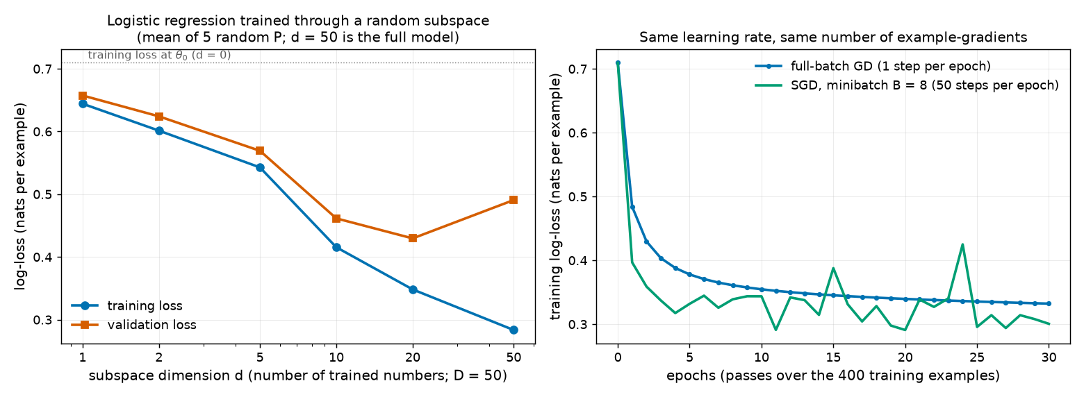
Logistic regression: noisy minibatches and the reach of a subspace¶
Logistic regression is a model for yes/no labels. Given an input vector \(x\in\mathbb R^{50}\), it predicts that the label is 1 with probability \(\sigma(\theta\cdot x)\), where \(\sigma(z)=1/(1+e^{-z})\) squeezes any number into \((0,1)\). Its loss is the log-loss of Chapter 6: \(-\ln\) of the probability given to the actual label, in nats. Here \(\theta\) has \(D=50\) entries.
We generated synthetic data in which the labels depend on only 5 hidden factors, mixed into all 50 inputs plus noise: \(m=400\) training examples and 20,000 validation examples (output [5]). We built this low-dimensional structure on purpose; it is a toy, not evidence about GPT-2.
Minibatch noise. At the starting point the full gradient has length 1.0963. Minibatch gradients scatter around it with mean squared error 12.6040, 1.5742 and 0.1969 for batch sizes 1, 8 and 64 — the formula \(\sigma^2/|\mathcal B|\) predicts 12.6046, 1.5756 and 0.1969 (output [5]).
SGD versus GD at equal cost. Both use learning rate 0.2707 and process 400 example-gradients per epoch. Full-batch GD takes 1 step per epoch; SGD with batch size 8 takes 50 cheaper, noisier steps. From a training loss of 0.7094:
- after 1 epoch: GD 0.4840, SGD 0.3968;
- after 5 epochs: GD 0.3779, SGD 0.3320;
- after 30 epochs: GD 0.3322, SGD 0.3006 (output [5]).
SGD gets further for the same work, but its curve jumps up and down (figure, right).
Training through random subspaces. Now train \(\theta=\theta_0+Pw\) with a random \(P\) of shape \(50\times d\) with orthonormal columns, by GD until the gradient vanishes. Each row is the mean over 5 random \(P\) (output [6]). At \(\theta_0\) itself the losses are 0.7094 (training) and 0.7165 (validation).
| \(d\) | training loss (nats/example) | validation loss (nats/example) |
|---|---|---|
| 1 | 0.6442 | 0.6574 |
| 2 | 0.6013 | 0.6241 |
| 5 | 0.5427 | 0.5692 |
| 10 | 0.4154 | 0.4615 |
| 20 | 0.3482 | 0.4296 |
| 50 (full model) | 0.2835 | 0.4907 |
The training loss falls steadily as \(d\) grows: more freedom, better fit. The validation loss is best at \(d=20\) (0.4296). The full model has the lowest training loss, 0.2835, but a worse validation loss, 0.4907: it overfits (Chapter 2). Fewer trained numbers can mean less overfitting. The paper builds on a related idea: fewer, compressible trained numbers mean a shorter description and a tighter bound (Chapter 14).
A seed instead of a million numbers¶
From output [7]: one million float32 normal numbers from seed 1234 are reproduced exactly (same SHA-256 fingerprint); they take 4,000,000 bytes, the seed 8. For GPT-2 small's 123,689,472 parameters, \(\theta_0\) written out is \(3.958\times10^{9}\) bits; the seed is 64 bits.
Going deeper¶
Everything in this section is MY EXPLANATION unless tagged.
The collapsible blocks above sit next to the ideas they deepen:
- the gradient as the steepest-ascent direction (under "The gradient");
- exact convergence of GD on a bowl (under "Gradient descent and the learning rate");
- unbiasedness and \(1/|\mathcal B|\) noise of minibatch gradients (under "Stochastic gradient descent");
- Adam's bias correction and AdamW's decoupling (under "Adam, weight decay and AdamW");
- the multivariable chain rule, proved, and backpropagation by hand (under "The chain rule");
- the reparameterization gradient and projected GD (under "Reparameterization");
- what a seed pins down (under "Random initialization").
Two more follow.
Going deeper: the descent lemma — a safe learning rate for any smooth loss
Assumption. The gradient changes at most \(\Lambda\) per unit of distance: \(\lVert\nabla\mathcal L(x)-\nabla\mathcal L(y)\rVert\le\Lambda\lVert x-y\rVert\) for all \(x,y\). For the bowl, \(\Lambda=2\max_kq_k=20\).
Lemma. \(\mathcal L(y)\le\mathcal L(x)+\nabla\mathcal L(x)\cdot(y-x)+\tfrac{\Lambda}{2}\lVert y-x\rVert^2\).
Proof. Let \(\varphi(\tau)=\mathcal L\big(x+\tau(y-x)\big)\) for \(\tau\in[0,1]\). By the chain rule, \(\varphi'(\tau)=\nabla\mathcal L\big(x+\tau(y-x)\big)\cdot(y-x)\). The fundamental theorem of calculus gives \(\mathcal L(y)-\mathcal L(x)=\varphi(1)-\varphi(0)=\int_0^1\varphi'(\tau)\,d\tau\). Subtract \(\nabla\mathcal L(x)\cdot(y-x)=\int_0^1\nabla\mathcal L(x)\cdot(y-x)\,d\tau\):
using Cauchy–Schwarz and the assumption with distance \(\tau\lVert y-x\rVert\). \(\square\)
Consequence. Put \(x=\theta^{(t)}\), \(y=\theta^{(t)}-\eta\nabla\mathcal L(\theta^{(t)})\) and write \(\gamma=\lVert\nabla\mathcal L(\theta^{(t)})\rVert\):
For \(0<\eta<2/\Lambda\) every step lowers the loss unless the gradient is already zero. For the bowl, \(2/\Lambda=0.1\), matching the exact analysis. At \(\eta=2/\Lambda\) the guarantee is gone — the bouncing at \(\eta=0.1\) in output [1] sits exactly on that edge. Summing the inequality over steps also shows that the gradients must shrink toward zero when \(\mathcal L\) is bounded below; it does not show that GD reaches the lowest possible loss.
Going deeper: multiplying by P and Pᵀ without storing P
A dense \(P\) for GPT-2 small (\(D=123{,}689{,}472\)) and \(d=50{,}000\) would hold \(6.184\times10^{12}\) numbers, or 24.7 TB in float32 (output [7]). Training needs \(Pw\) in every forward pass and \(P^\top\nabla_\theta\mathcal L\) in every backward pass, so \(P\) must be usable without being stored.
[SOURCE: authors' code, RandomMultiply in projectors.py] One option in the code regenerates the Gaussian
matrix chunk by chunk from its seed, in the forward pass to compute \(Pw\) and again in the backward pass to compute
\(P^\top g\). The same seed guarantees that both passes use the same matrix.
MY EXPLANATION The paper's main projector instead has Kronecker structure, \(P=Q_1\otimes Q_2\), so only the two small factors are stored and products are computed with the vec trick of Chapter 8. Chapter 18 covers it (and erratum E08 on the two constructions).
Common misconceptions¶
- Misconception: Gradient descent finds the best possible parameters. — Actually: it walks downhill until the slope (nearly) vanishes. For non-bowl-shaped losses that may be one valley among many. Through a reparameterization it finds the best point of the slice only: 14.54545 instead of 0 in the worked example.
- Misconception: A larger learning rate always trains faster. — Actually: past a threshold the steps overshoot and the loss grows. On the bowl, \(\eta=0.10\) leaves the loss stuck at 10 and \(\eta=0.11\) sends it to \(8.282\times10^{8}\) after 50 steps.
- Misconception: A minibatch gradient is a biased shortcut. — Actually: it is right on average; only its noise depends on the batch size, falling like \(1/|\mathcal B|\) (12.6040 → 1.5742 from 1 to 8 examples in output [5]).
- Misconception: Training in a subspace gives the same model, only cheaper. — Actually: it restricts which models can be reached. In the logistic example the training loss is 0.6442 with \(d=1\) against 0.2835 for the full model. That restriction is the point: it is what makes the result short to describe.
- Misconception: A random initialization with 123,689,472 numbers costs \(3.958\times10^{9}\) bits in the bound. — Actually: a seed fixed in advance plus fixed code reproduce it exactly; the paper counts it as part of the architecture. Only a seed chosen after seeing the data would cost bits (\(\log_2 k\) for the best of \(k\)).
- Misconception: The bound depends on how the model was trained (optimizer, learning rate, number of steps). — Actually: the bound needs only the final hypothesis and its description length, with a prior fixed before the data. Any search procedure is allowed. (The paper still pays 1.585 bits for the learning rate — harmless.)
- Misconception: The paper's bound needs validation data. — Actually: it uses only training data; that is its whole point. Validation numbers (Table 2) are reported separately, as a sanity check.
Self-test¶
Q1. In the worked example, why does \(\eta=0.05\) put \(\theta_2\) exactly at \(-1\) after one step, and what is the largest learning rate for which gradient descent still converges? What happens at exactly that value?
Answer
The error \(\theta_2+1\) is multiplied by \(1-2\eta q_2=1-2\cdot0.05\cdot10=0\) in one step, so it vanishes at once. Convergence needs \(|1-2\eta q_k|<1\) for both coordinates, i.e. \(\eta<1/\max(1,10)=0.1\). At \(\eta=0.1\) the factor for \(\theta_2\) is \(-1\): the error flips sign forever, \(\theta_2\) bounces between 0 and \(-2\), and the loss stays at 10 (output [1]).
Q2. Train the bowl through \(\theta=\theta_0+Pw\) with \(\theta_0=(0,0)\), \(P=(1,1)^\top/\sqrt2\). At \(w=0.5\) the gradient with respect to \(\theta\) is \((-5.29289,\,27.07107)\). What is \(d\mathcal L/dw\), and in which direction will a gradient-descent step move \(w\)?
Answer
\(d\mathcal L/dw=P^\top\nabla_\theta\mathcal L=(-5.29289+27.07107)/\sqrt2=15.399495\), which equals the finite difference in output [2] (and \(11w+14/\sqrt2\) at \(w=0.5\)). It is positive, so the step \(w\leftarrow w-\eta\cdot15.399495\) decreases \(w\), toward the best point \(w^\star=-0.89995\).
Q3. The paper's \(\theta_0\) for GPT-2 small consists of over a hundred million random numbers. Why does the compressed size \(C(h)\) not include them? What would change if the authors had trained with 1,000 different seeds and reported the best bound?
Answer
\(\theta_0\) (and \(P\)) come from a pseudo-random generator started from a seed that was fixed, together with the code, before any training data were seen. A decoder that knows the architecture can regenerate them bit for bit, so they are part of the architecture, which the paper gives to the decoder for free; nothing about them depends on the data, so the prior can be fixed in advance. Picking the best of 1,000 seeds is a data-dependent choice: the prior must spread over the 1,000 options, costing \(\log_2 1000=9.966\) extra bits (output [7]) — small, but owed. The other seed, used only to draw minibatches, steers the search and costs nothing.
Code for this chapter¶
Run it from the project root:
.venv/Scripts/python explainer/code/ch07_gd.py
Source: ch07_gd.py
"""Chapter 7 demo: training by gradient descent, through a reparameterization, from a seed.

Claims illustrated (all [MY EXPLANATION] unless marked [PAPER] / [SOURCE]):
  [1] Gradient descent (GD) on L(t1,t2) = (t1-3)^2 + 10 (t2+1)^2 from (0,0) with learning rate 0.05:
      first iterates and losses; the learning rate must stay below 0.1 (= 1 / largest coefficient) or GD fails.
  [2] The same loss trained through theta = theta0 + P w with theta0 = (0,0), P = (1,1)^T / sqrt(2) (D = 2, d = 1):
      the best reachable loss is 1760/121 = 14.545 (full space: 0). The reparameterization gradient
      dL/dw = P^T grad_theta L is checked by finite differences, and the general rule J^T grad for a nonlinear map.
  [3] Backpropagation (the chain rule) on a 2-2-1 tanh network, by hand, vs torch autograd vs finite differences.
  [4] Adam and AdamW written out by hand agree with torch.optim.Adam / AdamW; Adam's first step is
      lr * sign(gradient); decoupled weight decay shrinks a parameter by (1 - lr*lambda) per step
      ([PAPER App. E] lambda = 1e-2, eps = 1e-6, learning rates {2e-4, 5e-3, 5e-5}).
  [5] Minibatch gradients (logistic regression, D = 50) are unbiased and their mean squared error is
      sigma^2 / B; SGD with batch size 8 ([PAPER App. E] batch size) vs full-batch GD at equal cost.
  [6] Logistic regression trained through random subspaces of dimension d in {1,2,5,10,20,50}: training and
      validation loss vs d (preview of Chapter 18), mean over 5 random subspaces each.
  [7] Seeds: 1,000,000 Gaussian numbers regenerated bit-for-bit from seed 1234; 4,000,000 bytes vs 8 bytes;
      the same seed in a different generator gives different numbers; cost of picking the best of 1,000 seeds.
  [8] Flatten / unflatten round trip for the network of [3]; [SOURCE nanoGPT prepare.py] validation split.

Writes outputs/ch07_gd.txt, docs/assets/fig/ch07_gd_paths.png and docs/assets/fig/ch07_subspace_logreg.png.
Runtime: about 20 s on a laptop CPU (mostly importing torch and the subspace sweep).
"""
import hashlib
import math
import sys
from pathlib import Path

import numpy as np

HERE = Path(__file__).resolve().parent
sys.path.insert(0, str(HERE))
import pacbound  # noqa: E402

import matplotlib  # noqa: E402
matplotlib.use("Agg")
import matplotlib.pyplot as plt  # noqa: E402
import torch  # noqa: E402

torch.set_num_threads(1)
OUT_TXT = HERE / "outputs" / "ch07_gd.txt"
FIG_DIR = HERE.parent / "docs" / "assets" / "fig"
OUT_FIG1 = FIG_DIR / "ch07_gd_paths.png"
OUT_FIG2 = FIG_DIR / "ch07_subspace_logreg.png"
OUT_TXT.parent.mkdir(parents=True, exist_ok=True)
FIG_DIR.mkdir(parents=True, exist_ok=True)

BLUE, VERM, GREEN, PINK, ORANGE, SKY = "#0072B2", "#D55E00", "#009E73", "#CC79A7", "#E69F00", "#56B4E9"
lines = []


def out(s=""):
    lines.append(s)


out("Chapter 7 demo (numpy + torch CPU; every random draw comes from a fixed seed)")

# =====================================================================================
# [1] Gradient descent on a 2-parameter quadratic
# =====================================================================================
C = np.array([3.0, -1.0])          # location of the minimum
A = np.array([1.0, 10.0])          # coefficients: L = sum_k A_k (t_k - C_k)^2


def quad_loss(t):
    return float(np.sum(A * (np.asarray(t) - C) ** 2))


def quad_grad(t):
    return 2.0 * A * (np.asarray(t) - C)


def gd(t0, lr, steps):
    path = [np.array(t0, float)]
    for _ in range(steps):
        path.append(path[-1] - lr * quad_grad(path[-1]))
    return np.array(path)


LR = 0.05
path_gd = gd([0.0, 0.0], LR, 200)
out("[1] GD on L(t1,t2) = (t1-3)^2 + 10 (t2+1)^2, start (0,0), learning rate 0.05; gradient = (2(t1-3), 20(t2+1))")
out("    step   theta1    theta2    gradient            loss")
for t in list(range(6)) + [50]:
    g = quad_grad(path_gd[t])
    out(f"    {t:4d}  {path_gd[t][0]:8.5f}  {path_gd[t][1]:8.5f}   ({g[0]:7.4f}, {g[1]:7.4f})  {quad_loss(path_gd[t]):.6g}")
assert abs(quad_loss(path_gd[1]) - 7.29) < 1e-12 and path_gd[1][1] == -1.0
steps_1e6 = int(np.argmax([quad_loss(p) < 1e-6 for p in path_gd]))
out(f"    loss first below 1e-6 at step {steps_1e6}; per-step shrink factors |1 - 2*lr*A_k| = "
    f"{abs(1 - 2 * LR * A[0]):.2f} (theta1), {abs(1 - 2 * LR * A[1]):.2f} (theta2)")
sweep = []
for lr in [0.01, 0.05, 0.09, 0.10, 0.11]:
    sweep.append(f"{lr:.2f} -> {quad_loss(gd([0, 0], lr, 50)[-1]):.4g}")
out("    loss after 50 steps by learning rate (stable only if lr < 1/max A_k = 0.1): " + "; ".join(sweep[:3]))
out("      " + "; ".join(sweep[3:]) + "   (0.10: theta2 bounces between 0 and -2 forever; 0.11: diverges)")

# =====================================================================================
# [2] Reparameterization theta = theta0 + P w
# =====================================================================================
TH0 = np.zeros(2)
P = np.array([[1.0], [1.0]]) / math.sqrt(2.0)
w_star = -14.0 / (11.0 * math.sqrt(2.0))       # solves 11 w + 14/sqrt(2) = 0
best_line = quad_loss(TH0 + P[:, 0] * w_star)
assert abs(best_line - 1760.0 / 121.0) < 1e-12


def sub_grad(w):                                # dL/dw = P^T grad_theta L
    return float(P[:, 0] @ quad_grad(TH0 + P[:, 0] * w))


w_path = [0.0]
for _ in range(200):
    w_path.append(w_path[-1] - LR * sub_grad(w_path[-1]))
w_path = np.array(w_path)
sub_path = TH0 + np.outer(w_path, P[:, 0])
out("[2] Same loss through theta = theta0 + P w, theta0 = (0,0), P = (1,1)^T/sqrt(2): D = 2 numbers, d = 1 trained")
out(f"    best w* = -14/(11 sqrt 2) = {w_star:.5f} -> theta = ({TH0[0] + P[0, 0] * w_star:.5f}, "
    f"{TH0[1] + P[1, 0] * w_star:.5f}); best loss on the line = 1760/121 = {best_line:.5f} (full space: 0)")
g_star = quad_grad(TH0 + P[:, 0] * w_star)
assert abs(float(P[:, 0] @ g_star)) < 1e-12
out(f"    full gradient at that point = ({g_star[0]:.5f}, {g_star[1]:.5f}): not zero, but P^T grad = 0 "
    f"(perpendicular to the line)")
out(f"    GD on w (lr 0.05): w_1..w_3 = {w_path[1]:.5f}, {w_path[2]:.5f}, {w_path[3]:.5f}; "
    f"loss {quad_loss(sub_path[0]):.4f} -> {quad_loss(sub_path[1]):.4f} -> {quad_loss(sub_path[3]):.4f} "
    f"-> {quad_loss(sub_path[20]):.5f} (step 20)")
w_chk, h = 0.5, 1e-6
th_chk = TH0 + P[:, 0] * w_chk
g_th = quad_grad(th_chk)
fd = (quad_loss(TH0 + P[:, 0] * (w_chk + h)) - quad_loss(TH0 + P[:, 0] * (w_chk - h))) / (2 * h)
assert abs(fd - sub_grad(w_chk)) < 1e-6
out(f"    check at w = 0.5: grad_theta L = ({g_th[0]:.5f}, {g_th[1]:.5f}); P^T grad = {sub_grad(w_chk):.6f}; "
    f"finite difference = {fd:.6f}")


def f_nl(w):                                    # an arbitrary nonlinear map R^2 -> R^2
    return TH0 + np.array([w[0] * w[1], w[0] - w[1] ** 2])


def jac_nl(w):
    return np.array([[w[1], w[0]], [1.0, -2.0 * w[1]]])


w_nl = np.array([0.7, -0.4])
g_formula = jac_nl(w_nl).T @ quad_grad(f_nl(w_nl))
g_fd = np.array([(quad_loss(f_nl(w_nl + h * e)) - quad_loss(f_nl(w_nl - h * e))) / (2 * h) for e in np.eye(2)])
assert np.max(np.abs(g_formula - g_fd)) < 1e-5
out(f"    nonlinear map theta = (w1 w2, w1 - w2^2) at w = (0.7,-0.4): J^T grad = ({g_formula[0]:.5f}, "
    f"{g_formula[1]:.5f}), finite diff. = ({g_fd[0]:.5f}, {g_fd[1]:.5f})")
dirs = {"(1,1)/sqrt2": np.array([1.0, 1.0]), "random (seed 0)": np.random.default_rng(0).standard_normal(2),
        "(3,-1)/sqrt10": np.array([3.0, -1.0])}
best_by_dir = []
for name, u in dirs.items():
    u = u / np.linalg.norm(u)
    w_b = float(np.sum(A * u * C) / np.sum(A * u * u))   # minimizer of sum A_k (w u_k - C_k)^2
    best_by_dir.append(f"{name}: {quad_loss(w_b * u):.4f}")
out("    best loss along other lines through theta0: " + "; ".join(best_by_dir))

# =====================================================================================
# [3] Backpropagation on a 2-2-1 tanh network
# =====================================================================================
x_in, y_tg = np.array([1.0, 2.0]), 1.0
W1 = np.array([[0.5, -0.25], [0.8, 0.2]]); b1 = np.array([0.0, -0.1])   # z1 = 0 exactly in binary
W2 = np.array([[1.0, -0.5]]); b2 = np.array([0.2])


def net_loss(W1, b1, W2, b2):
    a = np.tanh(W1 @ x_in + b1)
    return 0.5 * float((W2 @ a + b2)[0] - y_tg) ** 2


z = W1 @ x_in + b1
a = np.tanh(z)
yhat = float((W2 @ a + b2)[0])
loss_net = 0.5 * (yhat - y_tg) ** 2
d_y = yhat - y_tg                               # dLoss/dyhat
gW2 = d_y * a[None, :] + 0.0; gb2 = np.array([d_y])   # "+ 0.0" prints (-1.2)*0 as 0, not -0
d_a = W2[0] * d_y                               # dLoss/da = W2^T d_y
d_z = d_a * (1.0 - a ** 2)                      # tanh'(z) = 1 - tanh(z)^2
gW1 = np.outer(d_z, x_in); gb1 = d_z
params = [W1, b1, W2, b2]
manual = [gW1, gb1, gW2, gb2]
tp = [torch.tensor(p, dtype=torch.float64, requires_grad=True) for p in params]
tl = 0.5 * ((tp[2] @ torch.tanh(tp[0] @ torch.tensor(x_in) + tp[1]) + tp[3])[0] - y_tg) ** 2
tl.backward()
diff_torch = max(float(np.max(np.abs(g - t.grad.numpy()))) for g, t in zip(manual, tp))
diff_fd = 0.0
for k, p in enumerate(params):
    for idx in np.ndindex(p.shape):
        pp = [q.copy() for q in params]; pm = [q.copy() for q in params]
        pp[k][idx] += h; pm[k][idx] -= h
        diff_fd = max(diff_fd, abs((net_loss(*pp) - net_loss(*pm)) / (2 * h) - manual[k][idx]))
assert diff_torch < 1e-12 and diff_fd < 1e-8
out("[3] Backprop, network x(2) -> z = W1 x + b1 -> a = tanh z -> yhat = W2 a + b2, loss = (yhat - y)^2/2, x = (1,2), y = 1")
out("    W1 = [[0.5, -0.25], [0.8, 0.2]], b1 = (0, -0.1), W2 = [[1, -0.5]], b2 = 0.2")
out(f"    forward: z = ({z[0]:.4f}, {z[1]:.4f}), a = ({a[0]:.6f}, {a[1]:.6f}), yhat = {yhat:.6f}, loss = {loss_net:.6f}")
out(f"    backward: dL/dyhat = {d_y:.6f}; dL/dW2 = ({gW2[0, 0]:.6f}, {gW2[0, 1]:.6f}); dL/da = ({d_a[0]:.6f}, "
    f"{d_a[1]:.6f}); dL/dz = ({d_z[0]:.6f}, {d_z[1]:.6f})")
out(f"    dL/dW1 = [[{gW1[0, 0]:.6f}, {gW1[0, 1]:.6f}], [{gW1[1, 0]:.6f}, {gW1[1, 1]:.6f}]]; "
    f"max |hand - torch autograd| = {diff_torch:.1e}; max |hand - finite diff.| = {diff_fd:.1e}")

# =====================================================================================
# [4] Adam and AdamW, by hand vs torch
# =====================================================================================


def adamw_numpy(t0, lr, steps, b1=0.9, b2=0.999, eps=1e-8, wd=0.0):
    th = np.array(t0, float); u = np.zeros_like(th); s = np.zeros_like(th); path = [th.copy()]
    for t in range(1, steps + 1):
        g = quad_grad(th)
        th = th * (1.0 - lr * wd)                      # decoupled weight decay (AdamW)
        u = b1 * u + (1 - b1) * g                      # running mean of gradients
        s = b2 * s + (1 - b2) * g * g                  # running mean of squared gradients
        uh, sh = u / (1 - b1 ** t), s / (1 - b2 ** t)  # bias correction
        th = th - lr * uh / (np.sqrt(sh) + eps)
        path.append(th.copy())
    return np.array(path)


def adamw_torch(t0, lr, steps, eps=1e-8, wd=0.0, decoupled=True):
    th = torch.tensor(t0, dtype=torch.float64, requires_grad=True)
    opt = (torch.optim.AdamW if decoupled else torch.optim.Adam)([th], lr=lr, betas=(0.9, 0.999), eps=eps,
                                                                weight_decay=wd)
    res = [th.detach().numpy().copy()]
    a_t, c_t = torch.tensor(A, dtype=torch.float64), torch.tensor(C, dtype=torch.float64)
    for _ in range(steps):
        opt.zero_grad()
        torch.sum(a_t * (th - c_t) ** 2).backward()
        opt.step()
        res.append(th.detach().numpy().copy())
    return np.array(res)


path_adam = adamw_numpy([0, 0], 0.1, 300)
diff_adam = float(np.max(np.abs(path_adam - adamw_torch([0.0, 0.0], 0.1, 300, decoupled=False))))
p_w = adamw_numpy([0, 0], 0.1, 300, eps=1e-6, wd=1e-2)
diff_adamw = float(np.max(np.abs(p_w - adamw_torch([0.0, 0.0], 0.1, 300, eps=1e-6, wd=1e-2))))
assert diff_adam < 1e-12 and diff_adamw < 1e-12
out("[4] Adam (betas 0.9, 0.999; eps 1e-8) on the [1] loss, lr 0.1. First gradient (-6, 20); first step = lr*sign(g)")
out(f"    theta_1 = ({path_adam[1][0]:.6f}, {path_adam[1][1]:.6f}), theta_2 = ({path_adam[2][0]:.6f}, "
    f"{path_adam[2][1]:.6f}), theta_3 = ({path_adam[3][0]:.6f}, {path_adam[3][1]:.6f})")
out(f"    loss after 100 / 300 steps: {quad_loss(path_adam[100]):.4g} / {quad_loss(path_adam[300]):.4g};  max |by hand - "
    f"torch Adam| = {diff_adam:.1e}; AdamW (wd 1e-2, eps 1e-6) vs torch AdamW: {diff_adamw:.1e}")
out(f"    [PAPER App. E] AdamW weight decay lambda = 1e-2: with zero gradient a weight is multiplied by (1 - lr*lambda)"
    " each step:")
wd_rows = []
for lr in pacbound.LR_GRID:
    f = 1 - lr * 1e-2
    wd_rows.append(f"lr {lr:g}: factor {f:.7f}, halves after {math.log(2) / -math.log(f):,.0f} steps")
out("      " + "; ".join(wd_rows))

# =====================================================================================
# [5] + [6] Logistic regression: minibatch noise, SGD vs GD, random subspaces
# =====================================================================================
D_LR, K_LAT, M_TR, N_VA, B_PAPER = 50, 5, 400, 20000, 8
rng = np.random.default_rng(1)
A_lat = rng.standard_normal((D_LR, K_LAT)) / math.sqrt(K_LAT)
v_lat = rng.standard_normal(K_LAT); v_lat *= 3.0 / np.linalg.norm(v_lat)
Zl = rng.standard_normal((M_TR + N_VA, K_LAT))
Xall = Zl @ A_lat.T + 0.5 * rng.standard_normal((M_TR + N_VA, D_LR))
yall = (rng.random(M_TR + N_VA) < 1.0 / (1.0 + np.exp(-Zl @ v_lat))).astype(float)
Xtr, ytr, Xva, yva = Xall[:M_TR], yall[:M_TR], Xall[M_TR:], yall[M_TR:]
theta0_lr = 0.1 * rng.standard_normal(D_LR)


def sigm(zz):
    return 1.0 / (1.0 + np.exp(-zz))


def lr_loss(th, X, y):        # mean log-loss in nats per example
    zz = X @ th
    return float(np.mean(np.logaddexp(0.0, zz) - y * zz))


def lr_grad(th, X, y):
    return X.T @ (sigm(X @ th) - y) / len(y)


g_full = lr_grad(theta0_lr, Xtr, ytr)
per_ex = Xtr * (sigm(Xtr @ theta0_lr) - ytr)[:, None]          # one gradient per training example
sig2 = float(np.mean(np.sum((per_ex - g_full) ** 2, axis=1)))
rng_mb = np.random.default_rng(2)
mb_rows = []
for B in [1, B_PAPER, 64]:
    idx = rng_mb.integers(0, M_TR, size=(20000, B))            # with replacement, like [PAPER App. E]
    gB = per_ex[idx].mean(axis=1)
    mse = float(np.mean(np.sum((gB - g_full) ** 2, axis=1)))
    assert abs(mse / (sig2 / B) - 1) < 0.05
    mb_rows.append(f"B={B}: {mse:.4f} (formula {sig2 / B:.4f})")
    if B == B_PAPER:
        bias_rel = float(np.linalg.norm(gB.mean(axis=0) - g_full) / np.linalg.norm(g_full))
out(f"[5] Logistic regression, D = {D_LR} weights, m = {M_TR} training / {N_VA:,} validation examples; loss in nats/example")
out(f"    at theta0: |full gradient| = {np.linalg.norm(g_full):.4f}; sigma^2 = mean |per-example grad - full grad|^2 = "
    f"{sig2:.4f}")
out("    mean |minibatch grad - full grad|^2 over 20,000 minibatches: " + "; ".join(mb_rows))
out(f"    average of the 20,000 B=8 minibatch gradients is off the full gradient by {100 * bias_rel:.2f}% (unbiased)")
L_smooth = float(np.linalg.eigvalsh(Xtr.T @ Xtr / M_TR).max() / 4.0)   # curvature bound of the log-loss
LR_LOG = 1.0 / L_smooth
EPOCHS = 30
th_gd = theta0_lr.copy(); th_sgd = theta0_lr.copy()
curve_gd, curve_sgd = [lr_loss(th_gd, Xtr, ytr)], [lr_loss(th_sgd, Xtr, ytr)]
rng_sgd = np.random.default_rng(3)
for ep in range(EPOCHS):
    th_gd = th_gd - LR_LOG * lr_grad(th_gd, Xtr, ytr)          # 1 step per epoch
    perm = rng_sgd.permutation(M_TR)
    for j in range(0, M_TR, B_PAPER):                          # M_TR / 8 = 50 steps per epoch
        bidx = perm[j:j + B_PAPER]
        th_sgd = th_sgd - LR_LOG * lr_grad(th_sgd, Xtr[bidx], ytr[bidx])
    curve_gd.append(lr_loss(th_gd, Xtr, ytr)); curve_sgd.append(lr_loss(th_sgd, Xtr, ytr))
out(f"    same lr = {LR_LOG:.4f}; training loss after 1 / 5 / {EPOCHS} epochs (one epoch = {M_TR} example-gradients),"
    f" starting from {curve_gd[0]:.4f}:")
out(f"      full-batch GD (1 step/epoch): {curve_gd[1]:.4f} / {curve_gd[5]:.4f} / {curve_gd[-1]:.4f};  "
    f"SGD, B = 8 ({M_TR // B_PAPER} steps/epoch): {curve_sgd[1]:.4f} / {curve_sgd[5]:.4f} / {curve_sgd[-1]:.4f}")

# --- [6] subspace sweep: theta = theta0 + P w, P = orthonormalized Gaussian D x d, trained to convergence by GD
D_LIST, REPS, STEPS = [1, 2, 5, 10, 20, 50], 5, 4000
rng_p = np.random.default_rng(4)
z0_tr = Xtr @ theta0_lr
res_sub = {}
for d in D_LIST:
    trs, vas, gns = [], [], []
    for _ in range(REPS):
        Pq, _ = np.linalg.qr(rng_p.standard_normal((D_LR, d)))   # orthonormal columns (Chapter 8)
        XP = Xtr @ Pq
        lr_d = 4.0 / float(np.linalg.eigvalsh(XP.T @ XP / M_TR).max())
        w = np.zeros(d)
        for it in range(STEPS):
            gw = XP.T @ (sigm(z0_tr + XP @ w) - ytr) / M_TR      # = P^T grad_theta (reparameterization rule)
            if it % 25 == 0 and np.linalg.norm(gw) < 1e-7:      # converged: stop early
                break
            w -= lr_d * gw
        th = theta0_lr + Pq @ w
        trs.append(lr_loss(th, Xtr, ytr)); vas.append(lr_loss(th, Xva, yva)); gns.append(float(np.linalg.norm(gw)))
    assert max(gns) < 1e-5
    res_sub[d] = (np.mean(trs), np.mean(vas), np.std(trs))
# torch check of the reparameterization gradient for one subspace
Pq_t = torch.tensor(np.linalg.qr(np.random.default_rng(5).standard_normal((D_LR, 10)))[0])
w_t = torch.zeros(10, dtype=torch.float64, requires_grad=True)
th_t = torch.tensor(theta0_lr) + Pq_t @ w_t
zz_t = torch.tensor(Xtr) @ th_t
torch.mean(torch.nn.functional.softplus(zz_t) - torch.tensor(ytr) * zz_t).backward()
diff_rep = float(np.max(np.abs(w_t.grad.numpy() - Pq_t.numpy().T @ lr_grad(theta0_lr, Xtr, ytr))))
assert diff_rep < 1e-12
out(f"[6] Same task, theta = theta0 + P w with random P (D = 50, orthonormal columns), GD to convergence, mean of "
    f"{REPS} random P")
out(f"    loss at theta0 (d = 0): train {lr_loss(theta0_lr, Xtr, ytr):.4f}, validation {lr_loss(theta0_lr, Xva, yva):.4f}")
out("       d   train loss (sd over P)   validation loss")
for d in D_LIST:
    out(f"    {d:4d}   {res_sub[d][0]:.4f}  ({res_sub[d][2]:.4f})         {res_sub[d][1]:.4f}")
out(f"    autograd w.grad vs P^T grad_theta (d = 10): max difference {diff_rep:.1e}")

# =====================================================================================
# [7] Seeds
# =====================================================================================
N_SEED = 1_000_000
r1 = np.random.default_rng(1234).standard_normal(N_SEED, dtype=np.float32)
r2 = np.random.default_rng(1234).standard_normal(N_SEED, dtype=np.float32)
r3 = np.random.default_rng(1235).standard_normal(N_SEED, dtype=np.float32)
h1, h2 = hashlib.sha256(r1.tobytes()).hexdigest()[:16], hashlib.sha256(r2.tobytes()).hexdigest()[:16]
assert np.array_equal(r1, r2) and h1 == h2
torch.manual_seed(1234); t1 = torch.randn(N_SEED)
torch.manual_seed(1234); t2 = torch.randn(N_SEED)
assert torch.equal(t1, t2)
D_GPT2 = pacbound.gpt2_params(12, 768)          # nanoGPT counting convention (as in Chapters 2 and 5)
out(f"[7] Seed 1234 -> 1,000,000 float32 Gaussians, generated twice: identical = {bool(np.array_equal(r1, r2))}, "
    f"SHA-256 prefixes {h1} / {h2}")
out(f"    seed 1235 instead: {int(np.sum(r1 == r3))} of 1,000,000 entries equal. torch generator, same seed: "
    f"identical = {bool(torch.equal(t1, t2))}")
out(f"    first 3 numbers, seed 1234: numpy ({r1[0]:.4f}, {r1[1]:.4f}, {r1[2]:.4f}) vs torch ({t1[0]:.4f}, "
    f"{t1[1]:.4f}, {t1[2]:.4f}) -> the generator is part of the description")
out(f"    storage: {N_SEED:,} x 4 bytes = {4 * N_SEED:,} bytes vs 8 bytes (64-bit seed) = factor {4 * N_SEED // 8:,}")
out(f"    GPT-2 small theta0: D = {D_GPT2:,} numbers (nanoGPT count) x 32 bits = {32 * D_GPT2:.3e} bits vs 64 bits")
out(f"    dense P for that D and d = 50,000: {D_GPT2 * 50_000:.3e} numbers = {4 * D_GPT2 * 50_000 / 1e12:.1f} TB "
    f"(float32) -> regenerate, never store")
out(f"    picking the best of 1,000 seeds after seeing data costs log2(1000) = {math.log2(1000):.3f} extra bits")

# =====================================================================================
# [8] Flatten / unflatten, paper settings, validation split
# =====================================================================================
shapes = [p.shape for p in params]
flat = np.concatenate([p.ravel() for p in params])
offs = np.cumsum([0] + [p.size for p in params])
unflat = [flat[offs[i]:offs[i + 1]].reshape(shapes[i]) for i in range(len(params))]
assert all(np.array_equal(p, q) for p, q in zip(params, unflat))
out(f"[8] flatten [W1 {shapes[0]}, b1 {shapes[1]}, W2 {shapes[2]}, b2 {shapes[3]}] -> vector of D = {flat.size}, "
    f"offsets {list(map(int, offs[:-1]))}; unflatten round trip exact: True")
out(f"    [PAPER App. E] batch {B_PAPER} x context {pacbound.CONTEXT} = {B_PAPER * pacbound.CONTEXT:,} tokens per "
    f"minibatch; learning-rate grid {pacbound.LR_GRID} = log2(3) = {math.log2(3):.3f} bits; "
    f"[PAPER App. D] fine-tuning: 5 epochs, lr 2e-5")
# [SOURCE authors' code, sources/ext/sublora]: config_sublora_train.yaml and the defaults in sublora_pipeline.py
ACCUM = 40
out(f"    [SOURCE authors' config] betas (0.9, 0.999); {ACCUM} accumulated minibatches of {B_PAPER} = "
    f"{ACCUM * B_PAPER} sequences per update; max 600,000 updates; no_decay_bias False; w starts at 0")
out("    [SOURCE authors' code defaults] linear warm-up 2,000 steps then cosine decay; gradient clipping at norm 1.0;"
    " seeds 137 (theta0, P), 1337 (batches)")
VAL_DOCS = 4007   # [SOURCE nanoGPT prepare.py] test_size=0.0005, seed=2357
out(f"    [SOURCE nanoGPT prepare.py] OpenWebText split (seed 2357): train m = {pacbound.M_DOCS:,} docs, "
    f"validation {VAL_DOCS:,} docs ({100 * VAL_DOCS / (VAL_DOCS + pacbound.M_DOCS):.3f}%)")
out(f"    one pass over {pacbound.OWT_TRAIN_TOKENS:,} train tokens in minibatches of 8 x 1024 tokens = "
    f"{pacbound.OWT_TRAIN_TOKENS / (B_PAPER * pacbound.CONTEXT):,.0f} steps")

# =====================================================================================
# Figures
# =====================================================================================
fig, (ax1, ax2) = plt.subplots(1, 2, figsize=(12, 4.8))
g1, g2 = np.meshgrid(np.linspace(-1.6, 4.2, 400), np.linspace(-2.4, 0.9, 400))
LL = (g1 - 3) ** 2 + 10 * (g2 + 1) ** 2
cs = ax1.contour(g1, g2, LL, levels=[0.25, 1, 2.5, 5, 10, 14.545, 20, 35, 55], colors="0.6", linewidths=0.8)
ax1.clabel(cs, fmt="%g", fontsize=8)
tline = np.linspace(-2.2, 1.2, 10)
ax1.plot(tline * P[0, 0], tline * P[1, 0], color=PINK, lw=1.2, ls="--",
         label=r"the line $\theta_0 + P w$ (all reachable $\theta$, d = 1)")
ax1.plot(path_gd[:40, 0], path_gd[:40, 1], "o-", color=BLUE, ms=3.5, lw=1.4, label="GD in full space (lr 0.05)")
ax1.plot(path_adam[:60, 0], path_adam[:60, 1], ".-", color=ORANGE, ms=3, lw=1.0, label="Adam (lr 0.1)")
ax1.plot(sub_path[:15, 0], sub_path[:15, 1], "s-", color=VERM, ms=4, lw=1.4, label="GD on w (lr 0.05)")
ax1.plot([3], [-1], "*", color=GREEN, ms=14, label="full minimum (3, -1), loss 0")
ax1.plot([sub_path[-1, 0]], [sub_path[-1, 1]], "X", color=VERM, ms=10, label="best on the line, loss 14.55")
ax1.set_xlabel(r"$\theta_1$ (parameter value)", fontsize=11)
ax1.set_ylabel(r"$\theta_2$ (parameter value)", fontsize=11)
ax1.set_title(r"Contours of $(\theta_1-3)^2 + 10(\theta_2+1)^2$ and three training paths", fontsize=11)
ax1.legend(fontsize=8.5, loc="lower right", framealpha=0.9)
ax1.set_xlim(-1.6, 4.2); ax1.set_ylim(-2.4, 0.9)
steps = np.arange(81)
ax2.semilogy(steps, [quad_loss(p) for p in path_gd[:81]], color=BLUE, lw=2, label="GD, full space (lr 0.05)")
ax2.semilogy(steps, [quad_loss(p) for p in path_adam[:81]], color=ORANGE, lw=1.6, label="Adam, full space (lr 0.1)")
ax2.semilogy(steps, [quad_loss(p) for p in sub_path[:81]], color=VERM, lw=2, label="GD on w (d = 1)")
ax2.axhline(best_line, color=VERM, lw=0.8, ls=":")
ax2.text(45, best_line * 1.25, "floor of the subspace: 14.545", color=VERM, fontsize=9)
ax2.set_xlabel("step t", fontsize=11)
ax2.set_ylabel("loss (log scale, loss units)", fontsize=11)
ax2.set_title("Loss per step", fontsize=11)
ax2.legend(fontsize=9, frameon=False, loc="lower left")
for ax in (ax1, ax2):
    ax.grid(alpha=0.25, lw=0.6); ax.tick_params(labelsize=10)
fig.tight_layout()
fig.savefig(OUT_FIG1, dpi=130)
plt.close(fig)

fig, (ax1, ax2) = plt.subplots(1, 2, figsize=(12, 4.4))
ax1.plot(D_LIST, [res_sub[d][0] for d in D_LIST], "o-", color=BLUE, lw=2, label="training loss")
ax1.plot(D_LIST, [res_sub[d][1] for d in D_LIST], "s-", color=VERM, lw=2, label="validation loss")
ax1.axhline(lr_loss(theta0_lr, Xtr, ytr), color="0.5", lw=0.8, ls=":")
ax1.text(1.05, lr_loss(theta0_lr, Xtr, ytr) + 0.006, r"training loss at $\theta_0$ (d = 0)", fontsize=9, color="0.35")
ax1.set_xscale("log"); ax1.set_xticks(D_LIST); ax1.set_xticklabels([str(d) for d in D_LIST])
ax1.set_xlabel("subspace dimension d (number of trained numbers; D = 50)", fontsize=11)
ax1.set_ylabel("log-loss (nats per example)", fontsize=11)
ax1.set_title("Logistic regression trained through a random subspace\n(mean of 5 random P; d = 50 is the full model)",
              fontsize=11)
ax1.legend(fontsize=10, frameon=False)
ep_axis = np.arange(EPOCHS + 1)
ax2.plot(ep_axis, curve_gd, "o-", color=BLUE, ms=3, lw=2, label="full-batch GD (1 step per epoch)")
ax2.plot(ep_axis, curve_sgd, "-", color=GREEN, lw=2, label="SGD, minibatch B = 8 (50 steps per epoch)")
ax2.set_xlabel("epochs (passes over the 400 training examples)", fontsize=11)
ax2.set_ylabel("training log-loss (nats per example)", fontsize=11)
ax2.set_title("Same learning rate, same number of example-gradients", fontsize=11)
ax2.legend(fontsize=10, frameon=False)
for ax in (ax1, ax2):
    ax.grid(alpha=0.25, lw=0.6); ax.tick_params(labelsize=10)
fig.tight_layout()
fig.savefig(OUT_FIG2, dpi=130)
plt.close(fig)
out(f"figures: docs/assets/fig/{OUT_FIG1.name}, docs/assets/fig/{OUT_FIG2.name}")

text = "\n".join(lines) + "\n"
print(text, end="")
OUT_TXT.write_text(text, encoding="utf-8")
Output:
Chapter 7 demo (numpy + torch CPU; every random draw comes from a fixed seed)
[1] GD on L(t1,t2) = (t1-3)^2 + 10 (t2+1)^2, start (0,0), learning rate 0.05; gradient = (2(t1-3), 20(t2+1))
    step   theta1    theta2    gradient            loss
       0   0.00000   0.00000   (-6.0000, 20.0000)  19
       1   0.30000  -1.00000   (-5.4000,  0.0000)  7.29
       2   0.57000  -1.00000   (-4.8600,  0.0000)  5.9049
       3   0.81300  -1.00000   (-4.3740,  0.0000)  4.78297
       4   1.03170  -1.00000   (-3.9366,  0.0000)  3.8742
       5   1.22853  -1.00000   (-3.5429,  0.0000)  3.13811
      50   2.98454  -1.00000   (-0.0309,  0.0000)  0.000239053
    loss first below 1e-6 at step 76; per-step shrink factors |1 - 2*lr*A_k| = 0.90 (theta1), 0.00 (theta2)
    loss after 50 steps by learning rate (stable only if lr < 1/max A_k = 0.1): 0.01 -> 1.194; 0.05 -> 0.0002391; 0.09 -> 2.37e-08
      0.10 -> 10; 0.11 -> 8.282e+08   (0.10: theta2 bounces between 0 and -2 forever; 0.11: diverges)
[2] Same loss through theta = theta0 + P w, theta0 = (0,0), P = (1,1)^T/sqrt(2): D = 2 numbers, d = 1 trained
    best w* = -14/(11 sqrt 2) = -0.89995 -> theta = (-0.63636, -0.63636); best loss on the line = 1760/121 = 14.54545 (full space: 0)
    full gradient at that point = (-7.27273, 7.27273): not zero, but P^T grad = 0 (perpendicular to the line)
    GD on w (lr 0.05): w_1..w_3 = -0.49497, -0.71771, -0.81795; loss 19.0000 -> 15.4475 -> 14.5824 -> 14.54545 (step 20)
    check at w = 0.5: grad_theta L = (-5.29289, 27.07107); P^T grad = 15.399495; finite difference = 15.399495
    nonlinear map theta = (w1 w2, w1 - w2^2) at w = (0.7,-0.4): J^T grad = (33.42400, 20.04800), finite diff. = (33.42400, 20.04800)
    best loss along other lines through theta0: (1,1)/sqrt2: 14.5455; random (seed 0): 3.8469; (3,-1)/sqrt10: 0.0000
[3] Backprop, network x(2) -> z = W1 x + b1 -> a = tanh z -> yhat = W2 a + b2, loss = (yhat - y)^2/2, x = (1,2), y = 1
    W1 = [[0.5, -0.25], [0.8, 0.2]], b1 = (0, -0.1), W2 = [[1, -0.5]], b2 = 0.2
    forward: z = (0.0000, 1.1000), a = (0.000000, 0.800499), yhat = -0.200250, loss = 0.720299
    backward: dL/dyhat = -1.200250; dL/dW2 = (0.000000, -0.960799); dL/da = (-1.200250, 0.600125); dL/dz = (-1.200250, 0.215566)
    dL/dW1 = [[-1.200250, -2.400499], [0.215566, 0.431131]]; max |hand - torch autograd| = 0.0e+00; max |hand - finite diff.| = 1.0e-10
[4] Adam (betas 0.9, 0.999; eps 1e-8) on the [1] loss, lr 0.1. First gradient (-6, 20); first step = lr*sign(g)
    theta_1 = (0.100000, -0.100000), theta_2 = (0.199897, -0.199588), theta_3 = (0.299618, -0.298414)
    loss after 100 / 300 steps: 0.0004605 / 2.274e-13;  max |by hand - torch Adam| = 4.4e-16; AdamW (wd 1e-2, eps 1e-6) vs torch AdamW: 8.9e-16
    [PAPER App. E] AdamW weight decay lambda = 1e-2: with zero gradient a weight is multiplied by (1 - lr*lambda) each step:
      lr 0.0002: factor 0.9999980, halves after 346,573 steps; lr 0.005: factor 0.9999500, halves after 13,863 steps; lr 5e-05: factor 0.9999995, halves after 1,386,294 steps
[5] Logistic regression, D = 50 weights, m = 400 training / 20,000 validation examples; loss in nats/example
    at theta0: |full gradient| = 1.0963; sigma^2 = mean |per-example grad - full grad|^2 = 12.6046
    mean |minibatch grad - full grad|^2 over 20,000 minibatches: B=1: 12.6040 (formula 12.6046); B=8: 1.5742 (formula 1.5756); B=64: 0.1969 (formula 0.1969)
    average of the 20,000 B=8 minibatch gradients is off the full gradient by 0.67% (unbiased)
    same lr = 0.2707; training loss after 1 / 5 / 30 epochs (one epoch = 400 example-gradients), starting from 0.7094:
      full-batch GD (1 step/epoch): 0.4840 / 0.3779 / 0.3322;  SGD, B = 8 (50 steps/epoch): 0.3968 / 0.3320 / 0.3006
[6] Same task, theta = theta0 + P w with random P (D = 50, orthonormal columns), GD to convergence, mean of 5 random P
    loss at theta0 (d = 0): train 0.7094, validation 0.7165
       d   train loss (sd over P)   validation loss
       1   0.6442  (0.0717)         0.6574
       2   0.6013  (0.0797)         0.6241
       5   0.5427  (0.0810)         0.5692
      10   0.4154  (0.0155)         0.4615
      20   0.3482  (0.0126)         0.4296
      50   0.2835  (0.0000)         0.4907
    autograd w.grad vs P^T grad_theta (d = 10): max difference 1.3e-16
[7] Seed 1234 -> 1,000,000 float32 Gaussians, generated twice: identical = True, SHA-256 prefixes d76a2dfd93ccaabf / d76a2dfd93ccaabf
    seed 1235 instead: 0 of 1,000,000 entries equal. torch generator, same seed: identical = True
    first 3 numbers, seed 1234: numpy (-1.9306, 2.7259, 1.5235) vs torch (-0.1117, -0.4966, 0.1631) -> the generator is part of the description
    storage: 1,000,000 x 4 bytes = 4,000,000 bytes vs 8 bytes (64-bit seed) = factor 500,000
    GPT-2 small theta0: D = 123,689,472 numbers (nanoGPT count) x 32 bits = 3.958e+09 bits vs 64 bits
    dense P for that D and d = 50,000: 6.184e+12 numbers = 24.7 TB (float32) -> regenerate, never store
    picking the best of 1,000 seeds after seeing data costs log2(1000) = 9.966 extra bits
[8] flatten [W1 (2, 2), b1 (2,), W2 (1, 2), b2 (1,)] -> vector of D = 9, offsets [0, 4, 6, 8]; unflatten round trip exact: True
    [PAPER App. E] batch 8 x context 1024 = 8,192 tokens per minibatch; learning-rate grid [0.0002, 0.005, 5e-05] = log2(3) = 1.585 bits; [PAPER App. D] fine-tuning: 5 epochs, lr 2e-5
    [SOURCE authors' config] betas (0.9, 0.999); 40 accumulated minibatches of 8 = 320 sequences per update; max 600,000 updates; no_decay_bias False; w starts at 0
    [SOURCE authors' code defaults] linear warm-up 2,000 steps then cosine decay; gradient clipping at norm 1.0; seeds 137 (theta0, P), 1337 (batches)
    [SOURCE nanoGPT prepare.py] OpenWebText split (seed 2357): train m = 8,009,762 docs, validation 4,007 docs (0.050%)
    one pass over 9,035,582,198 train tokens in minibatches of 8 x 1024 tokens = 1,102,976 steps
figures: docs/assets/fig/ch07_gd_paths.png, docs/assets/fig/ch07_subspace_logreg.png