15. Making the data i.i.d.: documents, not tokens¶
Where this fits
Prerequisites: Chapter 1 (independence, i.i.d., population, sampling with and without replacement, "fixed vs random"), Chapter 2 (data-generating process, empirical and expected risk), Chapter 4 (token, end-of-text token, OpenWebText, context window), Chapter 6 (bits per token, document-level vs token-level average), Chapter 9 (the three requirements of Hoeffding's inequality), Chapter 11 (Eq. 1). Used later by: Chapter 16 (prediction smoothing), Chapter 17 (the subsampling bound), Chapter 25 (Tables 1 and 4), Chapter 29 (critique). Purpose: decide what one "example" is when the data are text, show why tokens cannot play that role, and pin down which population the paper's bounds are actually about.
The problem this chapter solves¶
MY EXPLANATION The paper's main tool is Eq. (1) (Chapter 11). In words: the expected loss \(R(h)\) of a hypothesis \(h\) is at most its average training loss \(\hat R(h)\) plus a penalty. The penalty is
where \(\Delta\) is the width of the interval that contains every loss value, \(P(h)\) is the prior, \(\delta\) the failure probability and \(m\) the number of training examples.
The penalty shrinks like \(1/\sqrt m\). So the more examples, the tighter the bound. But the bound rests on Hoeffding's inequality, and that inequality needs the \(m\) losses to be independent (Chapter 9).
PAPER §1, p. 1 The paper lists this as its first challenge: a language model predicts tokens one after another, so its token predictions are not independent.
MY EXPLANATION The tempting move is to call every token an example. OpenWebText has about nine billion training tokens, so \(m\) would be enormous and the penalty tiny. This chapter shows that the move is wrong, by how much, and what the paper does instead: each whole document is one example.
Two questions follow, and the chapter answers both.
- Why are documents acceptable examples when tokens are not?
- Once documents are the examples, what exactly is the bound a statement about? Which population does \(R(h)\) average over?
Intuition (and where the analogy breaks)¶
Everything in this section is MY EXPLANATION.
Picture an essay contest. You want to know how good a grader's scoring rule is on essays in general.
Grading single sentences would be a mistake. The sentences of one essay share an author, a topic, a style and a vocabulary. If the first sentence is about tax law, so is the tenth. Two hundred sentences from five essays carry much less information than two hundred sentences from two hundred essays.
Whole essays from authors picked independently do not have this problem. What one author writes tells you nothing about what another, independently picked author writes. So you score each essay as one unit (average the sentence scores inside it), and then average over essays.
That is exactly the paper's move: token = sentence, document = essay.
Where it breaks.
- Nobody held a lottery. The analogy assumes authors were picked independently at random. The documents of OpenWebText were not drawn by lottery from "all web text". SOURCE: Radford et al. 2019, GPT-2 report, §2.1; Gokaslan & Cohen 2019, OpenWebText; neither is among the sources checked for this explainer As commonly described, they were collected from web pages linked in up-voted posts on the social-news site Reddit, then filtered and de-duplicated. MY EXPLANATION Independence of documents is an assumption about that process, not something anyone carried out.
- Contest entries influence each other. In a real contest, many essays respond to the same news story of the same week. Web pages do too (many pages about one event, many pages from one site). That is dependence between documents, and the analogy hides it.
- Equal votes. Scoring "per essay" gives a two-line note the same weight as a forty-page thesis. That is a choice, and it changes what "average score" means (erratum E28, below).
Precise definition¶
Everything in this section is MY EXPLANATION unless tagged.
Documents as the examples¶
PAPER §4.2, p. 4 The paper defines each example \(X_j\) in \(\hat R(h)\) to be an entire document drawn from the data-generating process that produced the corpus. The loss of \(h\) on a document is the negative log-likelihood of the whole document divided by its length.
A document is one unit of text in the corpus, such as one web page, turned into tokens. [SOURCE: nanoGPT
prepare.py] In OpenWebText as prepared by nanoGPT, each document is one web page's text, tokenized, with the
end-of-text token appended; documents are stored back to back in one long token stream, so the end-of-text tokens
mark the boundaries.
For a document \(X = (x_1,\dots,x_L)\) of \(L\) tokens, the loss is its bits per token (Chapter 6):
Here \(p_h(x_i \mid x_{<i})\) is the probability that the model assigns to the actual \(i\)-th token given all earlier tokens. (Strictly, \(p_h\) is the smoothed model, a mixture of the network's prediction with a uniform guess that keeps every probability away from zero; Chapter 16 makes this precise.) For top-\(k\) error the loss is the fraction of the document's tokens that miss the model's top \(k\) guesses.
Write \(\mathcal D\) for the distribution of the data-generating process: a random document is a draw \(X\sim\mathcal D\). The standing assumption of the document-level bound is that the training documents \(X_1,\dots,X_m\) are i.i.d. draws from \(\mathcal D\). Then
The first is the average over the training documents; the second is the average over a fresh random document.
Why documents meet Hoeffding's three requirements¶
Chapter 9 listed three requirements. Here is how per-document losses meet each one.
- Independence. If the documents are independent, then so are their losses \(R(h,X_1),\dots,R(h,X_m)\), for a fixed \(h\): each loss is computed from its own document only. (Proof in "Going deeper: functions of independent documents".) The tokens inside a document may depend on each other as strongly as they like. That dependence is sealed inside one number.
- A fixed interval. If every token's loss lies in \([a, a+\Delta]\), then so does their average, whatever the length \(L\). So every document's loss lies in the same interval of width \(\Delta\).
- \(h\) fixed in advance. Not provided by documents. Training chooses \(\hat h\) after seeing the data; the prior \(P(h)\) and the union bound handle that (Chapter 10, Chapter 11).
"Identically distributed" is used for a different purpose: it makes \(\mathbb E[\hat R(h)] = R(h)\), so that the quantity Hoeffding controls is the one we care about.
Paper erratum E28: every document weighs the same
PAPER §4.2, p. 4; §6.2, p. 7 The bound's risk is a per-document average of per-token losses.
MY EXPLANATION So \(R(h)\) is the expected bits per token of a random document, with a two-line page and a
forty-page page counting equally. It is not the expected loss of a random token of web text, which weights
documents by their length. Chapter 6 shows the two can differ a lot: on its synthetic corpus
the document-level average is 3.501 and the token-level average 2.918 bits per token (ch06_metrics.py). The
paper does not say which average its "Validation BPD" is, so bound and validation numbers may not be like with
like (erratum E28).
The population a bound is about¶
The population of a bound is the distribution from which the \(m\) examples are (assumed to be) i.i.d. draws. The expected risk \(R(h)\) is the average loss over that population, and the bound says nothing about anything else.
For the document-level bound the population is \(\mathcal D\): "a random document produced the way OpenWebText's documents were produced". It is not "all text", not chat, not code, not text written after the corpus was collected.
A document-level bound is Eq. (1) (or its subsampled form, Eq. (3), Chapter 17) with documents
as examples, \(m\) the number of training documents and population \(\mathcal D\). [SOURCE: nanoGPT prepare.py;
erratum E32] For OpenWebText \(m = 8{,}009{,}762\); the paper never states it.
Context chunks and the sequence-level bound¶
PAPER §4.2, pp. 4–5 The paper mentions an alternative example: a context chunk, a run of consecutive tokens whose length equals the model's context length. Chunks are natural because training already cuts the text into such pieces (a document can be longer than the context window). But chunks are not independent samples from the data-generating process. Valid bounds on chunks are still possible, says the paper, if one changes what the probability is over: no longer the random sampling from the data-generating process, but the random sampling of chunks from a fixed, finite dataset made by concatenating the documents.
PAPER App. B, p. 14 Concretely: chunks of 1,024 tokens (the context length) are taken from a non-overlapping chunking of OpenWebText.
MY EXPLANATION To say what "sampling from a fixed finite dataset" means we need one more term. The empirical distribution of a finite list \(c_1,\dots,c_M\) is the distribution of one item picked uniformly at random from the list: each position has probability \(1/M\), so an item that appears \(r\) times has probability \(r/M\). Its expected value is the plain average of the list. Drawing indices uniformly with replacement gives i.i.d. draws from it.
A sequence-level bound is the bound with context chunks as examples, \(m\) the number of chunks, and population the
empirical distribution of the corpus's chunks. [SOURCE: authors' code, data_size default; erratum E32]
\(m = 8{,}823{,}811\) chunks.
The paper's note on independence¶
Paraphrase of the Note on p. 5 (Satisfying the I.I.D. assumption)
PAPER §4.2, Note, p. 5 For document-level bounds the documents are sampled independently from the dataset. For sequence-level bounds OpenWebText is cut into context-length sequences, and sequences are sampled independently, so that one draw contains all tokens of one sequence. Whether draws from a set are independent depends on how one samples, not on what the set contains: even a set of near-identical items can be sampled independently. The elements are whole documents or whole sequences, never single tokens, and they are drawn independently.
MY EXPLANATION The note is correct about what it says: independence is a property of the sampling procedure. Step 4 of the worked example demonstrates it. But the paper's bound involves two different random draws, and the note's argument covers only one of them.
| Document level | Sequence level | |
|---|---|---|
| Training examples | 8,009,762 documents | 8,823,811 chunks of 1,024 tokens |
| What the \(m\)-term of Eq. (1)/(3) needs | training documents i.i.d. from \(\mathcal D\) | training chunks i.i.d. from the population |
| Is that provided by a sampler? | No: it is an assumption about how OpenWebText arose | No: the training data are all the chunks, not a random draw of them |
| What the \(n\)-term needs (Ch. 17) | subsample indices i.i.d. from the corpus | same |
| Is that provided by a sampler? | Yes, by construction (the authors' code) | Yes, by construction |
| Population, i.e. what \(R(h)\) averages over | \(\mathcal D\), a random fresh document | the corpus itself (its empirical distribution) |
(The \(n\)-term is the extra penalty for estimating \(\hat R(h)\) from \(n = 10{,}000\) randomly chosen documents instead of
all \(m\); Chapter 17 derives it. The authors' code draws those documents uniformly with
replacement [SOURCE: authors' code, sample_single_document].)
Paper erratum E54: the sequence-level bound is a statement about the training corpus
PAPER §4.2, pp. 4–5; App. B, p. 14 The paper says the sequence-level bound holds once the probability is reinterpreted as being over sampling chunks from the fixed, finite dataset, and that the resulting bounds differ in interpretation but are very close in value to the document-level ones.
MY EXPLANATION Under that reading the population is the empirical distribution of the corpus's chunks. Its expected risk \(R(h)\) is the average loss over all chunks of the corpus, and the model was trained on that very corpus. So \(R(h)\) is the full training loss \(\hat R(h)\), exactly, with no randomness involved. The \(m\)-term of Eq. (1) has no random draw behind it (the training set is the whole population, not \(m\) independent draws from it), and it is not needed: the inequality \(R(h)\le \hat R(h) + (\text{anything} \ge 0)\) holds with certainty. The only real probabilistic content is the \(n\)-term, which certifies the full training loss from a random subsample. The sequence-level numbers in Table 4 are therefore valid but are upper bounds on training loss, not on loss on new text. They say nothing about generalization (erratum E54). Proof in "Going deeper: sampling from a finite set".
Worked example with real numbers¶
Everything in this section is MY EXPLANATION unless tagged. All numbers come from ch15_iid.py (output blocks
[1]–[6]). Where δ appears it is 0.05 SOURCE: authors' code; erratum E31.
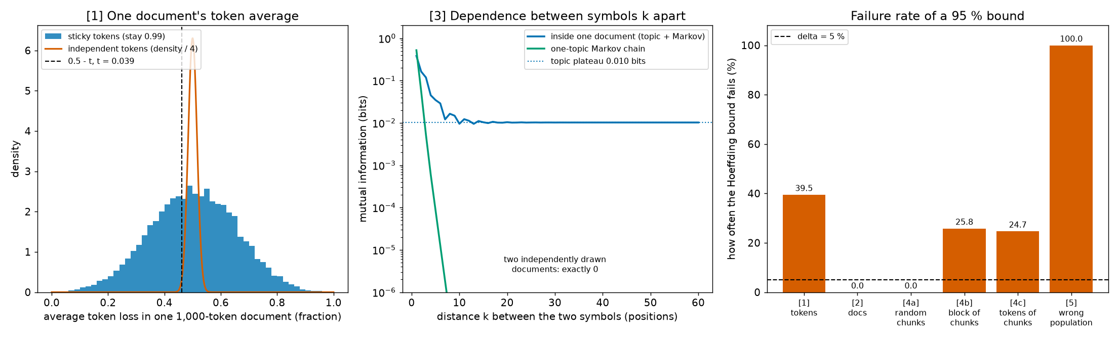
Step 1 — tokens as examples: the bound fails¶
Take the simplest possible "text" with dependent tokens. Each token has a loss of 0 or 1. The loss sequence is a sticky chain: each token copies the previous token's loss with probability "stay", and switches otherwise. The first token is 0 or 1 with probability 1/2 each, so every token has mean loss 0.5.
A document has \(L = 1{,}000\) tokens. If we pretend the tokens are independent, Hoeffding's inequality with \(m = L\) says the token average falls below \(0.5 - t\) with probability at most \(\delta\), where
The script simulates 10,000 documents for four values of "stay" and counts how often the average falls below \(0.5 - t\) (output [1]):
| stay | lag-1 correlation | sd of the token average | effective sample size | failure rate (should be ≤ 5 %) |
|---|---|---|---|---|
| 0.50 | 0.00 | 0.0158 | 1000.0 | 0.68 % |
| 0.90 | 0.80 | 0.0473 | 111.6 | 20.88 % |
| 0.99 | 0.98 | 0.1534 | 10.6 | 39.49 % |
| 1.00 | 1.00 | 0.5000 | 1.0 | 49.40 % |
At stay = 0.50 the tokens are independent, and the bound fails 0.68 % of the time, well inside 5 %. With dependence it fails 20.88 % or 39.49 % of the time. In the extreme (stay = 1) every token copies the first one, the average is 0 or 1, and the bound fails about half the time no matter how long the document is.
The effective sample size in the table is the number of independent tokens whose average would be exactly as variable as the average of the \(L\) dependent ones. A 1,000-token sticky document at stay 0.99 carries the information of 10.6 independent tokens. Hoeffding was told 1,000.
Step 2 — the same losses, documents as examples: the bound holds¶
Now keep the same sticky tokens but use the paper's recipe: each document's loss is its token average (a number in \([0,1]\), so \(\Delta = 1\)), and a dataset holds \(m = 100\) independently generated documents (output [2]).
- Hoeffding over \(m = 100\) documents: \(t = 0.1224\); over 1,000 simulated datasets the bound failed 0.00 % of the time.
- The same datasets, pretending they are 100,000 independent tokens: \(t = 0.0039\), failure rate 42.80 %.
Nothing about the data changed between the two lines. Only the choice of "example" changed. The honest margin (0.1224) is much wider than the dishonest one (0.0039): that width is the price of the dependence.
Step 3 — how far does dependence reach in text?¶
To measure dependence between two tokens we use mutual information: the average number of bits that knowing one symbol tells you about the other. It is 0 exactly when the two are independent, and positive otherwise (definition and proof in "Going deeper: mutual information").
The script builds synthetic text with 8 symbols. Each document first picks one of 4 "topics" at random; within the document, symbols then follow a Markov chain (each symbol depends on the previous one) whose transition table belongs to that topic. Output [3] gives the exact mutual information between symbols \(k\) positions apart:
| \(k\) | 1 | 2 | 3 | 5 | 10 | 20 | 50 | \(\to\infty\) |
|---|---|---|---|---|---|---|---|---|
| inside one document (topic + Markov), bits | 0.3827 | 0.1634 | 0.1185 | 0.0347 | 0.0095 | 0.0104 | 0.0102 | 0.0102 |
| one-topic Markov chain, bits | 0.5224 | 0.0557 | 0.0052 | 0.0001 | 0.0000 | 0.0000 | 0.0000 | 0.0000 |
Two lessons.
- A plain Markov chain forgets fast: by \(k = 10\) the dependence is below 0.0001 bits.
- A document-wide topic never lets go: the dependence levels off at 0.0102 bits however far apart the two symbols are. Real documents have topics, authors and styles. So dependence between tokens does not die out with distance inside a document, and no "skip every 100th token" trick would make tokens independent.
Between two independently drawn documents the mutual information is exactly 0. The script's estimate from 50,000 sampled pairs is 0.00070 bits, which matches the bias every such estimate has even for independent pairs (0.00071 bits).
Step 4 — independence comes from the sampler, not from the contents¶
Output [4] tests the paper's note. The script builds one fixed corpus: 3,000 documents stored grouped by topic (as real corpora are often stored grouped by source), 322,360 tokens, cut into 5,036 chunks of 64 tokens. The loss is the top-1 error of a predictor fixed before the corpus was made. The corpus average over chunks is \(R_{\text{corpus}} = 0.6594\).
Three ways to estimate \(R_{\text{corpus}}\) from \(n = 100\) chunks, each repeated 4,000 times, with the Hoeffding margin \(t = 0.1224\):
- (a) chunk indices drawn independently and uniformly, with replacement: failure rate 0.00 %;
- (b) one contiguous block of 100 chunks starting at a random place: failure rate 25.82 %;
- (c) the tokens of (a) treated as 6,400 independent examples (\(t = 0.0153\)): failure rate 24.68 %.
Same corpus, same contents, same chunks. Scheme (a) is valid because its indices are independent; (b) fails because one random starting point fixes all 100 chunks, which then share topics; (c) fails because tokens within a chunk are dependent. This is exactly what the note says.
Step 5 — the population is whatever the data were drawn from¶
Output [5] shows what independence does not buy. Suppose a "quality filter" keeps only documents of topics 0 and 1, and the corpus is drawn i.i.d. from the filtered stream. The expected per-document error is 0.4645 on filtered documents but 0.6555 on unfiltered ones.
Over 1,000 corpora of \(m = 100\) filtered documents, the bound "corpus average + 0.1224" failed 0.00 % of the time as a statement about filtered documents and 100.00 % of the time as a statement about unfiltered ones. The bound is perfectly valid. It is about the population the corpus came from, and about nothing else.
For OpenWebText that population is "pages of the kind OpenWebText collects". The bound transfers to other text only if that text looks like a fresh draw from the same process.
Step 6 — OpenWebText's two values of m¶
[SOURCE: nanoGPT prepare.py; authors' code defaults; erratum E32] Output [6]:
- OpenWebText has 8,013,769 documents. nanoGPT splits them at random into 8,009,762 training and 4,007 validation documents (validation = 0.050 %).
- The training split has 9,035,582,198 tokens, so the mean document has 1,128.1 tokens (including its end-of-text token).
- \(9{,}035{,}582{,}198 / 1{,}024 = 8{,}823{,}810.74\); rounded up this is 8,823,811, exactly the authors' sequence-level \(m\).
- \(m_{\text{seq}}/m_{\text{doc}} = 1.1016\): there are about 10 % more chunks than documents, because the mean document (1,128.1 tokens) is longer than one chunk (1,024). PAPER App. B, p. 14 The paper attributes the slightly larger \(m\) to some long documents, which is the same fact.
Because the \(m\)-term scales like \(1/\sqrt m\), it shrinks by the factor \(\sqrt{m_{\text{doc}}/m_{\text{seq}}} = 0.9528\)
at sequence level. For the paper's best bits-per-token model (compressed size 16.5325 KB from Fig. 2, read by
fig_extract.py; \(\alpha = 0.25\), so \(\Delta = 17.2020\) bits per token; \(n = 10{,}000\); δ = 0.05 SOURCE: authors'
code; no hyperparameter bits), the script finds:
| \(m\)-term (bits/token) | \(n\)-term (bits/token) | total penalty (bits/token) | |
|---|---|---|---|
| document level, \(m = 8{,}009{,}762\) | 1.3171 | 0.2106 | 1.5276 |
| sequence level, \(m = 8{,}823{,}811\) | 1.2548 | 0.2106 | 1.4654 |
The larger \(m\) lowers the penalty by 0.0622 bits per token.
PAPER Table 1, p. 6; Table 4, p. 14 The reported SubLoRA bounds differ (sequence minus document) by \(-0.24\) points for top-1 error, \(+0.28\) for top-10, \(+0.38\) for top-100 and \(-0.03\) bits per token for BPD (output [6]). MY EXPLANATION Two of the four sequence-level numbers are worse despite the larger \(m\), so the training-loss term must differ between the two evaluations as well. That matches the paper's remark that the differences come from the empirical risk evaluation. The two tables are not about the same quantity anyway: one is about fresh documents, the other about the training corpus (erratum E54).
Code note (not a paper erratum; see the Notes section of the errata page): the authors' chunk sampler covers 0.098 % of the corpus
[SOURCE: authors' code, sample_nonoverlapping_sequences in sublora_utils.py; call in
sublora_sublora_pipeline.py] The sequence-level sampler is called with data_size = 8,823,811 (the number of
chunks) and draws chunk indices below (data_size - 1) // block_size = 8,617, as if data_size were a token count.
Only the first 8,823,808 tokens can ever be drawn: 8,617 of the 8,823,811 chunks, or 0.098 % (output [6]).
MY EXPLANATION If Table 4 was computed with this released code, its subsample estimates the average over those 8,617 chunks, not over the corpus, and the \(n\)-term no longer certifies the corpus average. The first 8,617 chunks are probably a fair mix of documents (nanoGPT shuffles documents before the split), so the numbers may be close in practice, but the guarantee as stated does not cover them. This concerns the released code, not the paper's text; we cannot check which code produced Table 4.
Going deeper¶
Everything in this section is MY EXPLANATION unless tagged. The blocks below prove the facts the main text used: why the sticky average spreads so widely, why per-document losses are independent, what mutual information is, what sampling from a finite set gives, and what is random in each layer of the paper's bound.
Going deeper: the variance of a sticky average, and the effective sample size
Setup. Token states \(s_1,\dots,s_L\in\{0,1\}\) (the token losses). \(s_1\) is 0 or 1 with probability 1/2. For \(i\ge2\), a switch indicator \(e_i\) is 1 with probability \(q = 1-\text{stay}\) and 0 otherwise; the \(e_i\) are independent of each other and of \(s_1\); \(s_i = s_{i-1}\) if \(e_i = 0\) and \(s_i = 1-s_{i-1}\) if \(e_i = 1\).
Signs. Put \(y_i = 1 - 2s_i \in\{+1,-1\}\). A switch flips the sign, so \(y_i = y_{i-1}(1-2e_i)\) and, unrolling,
Each factor \(1-2e_l\) is \(+1\) with probability \(1-q\) and \(-1\) with probability \(q\); its mean is \(\rho = 1-2q = 2\,\text{stay}-1\).
Covariances. For \(i<j\), using \(y_i^2 = 1\),
where the expectation of a product of independent factors is the product of expectations (Chapter 1). Also \(\mathbb E[y_i] = \mathbb E[y_1]\cdot\rho^{i-1} = 0\). Hence \(\mathrm{Cov}(y_i,y_j) = \rho^{|i-j|}\), and since \(s_i = (1-y_i)/2\), \(\mathrm{Cov}(s_i,s_j) = \rho^{|i-j|}/4\). The lag-1 correlation is \(\rho\) (the table's second column).
Variance of the average. \(\bar s = \frac1L\sum_i s_i\). The variance of a sum is the sum of all pairwise covariances. There are \(L\) pairs with \(i = j\) and \(2(L-k)\) ordered pairs at distance \(k\ge1\):
With \(\rho = 0\) this is \(1/(4L)\), the i.i.d. value. The script evaluates it (column "sd theory", e.g. 0.1534 at stay 0.99) and the simulation agrees (0.1523).
Effective sample size. One token has variance \(1/4\). An average of \(n_{\text{eff}}\) independent tokens has variance \(1/(4n_{\text{eff}})\). Setting this equal to \(\operatorname{Var}[\bar s]\) gives \(n_{\text{eff}} = \frac{1}{4\operatorname{Var}[\bar s]}\). For long documents, \(\sum_{k\ge1}\rho^k = \rho/(1-\rho)\) while \(\sum_k k\rho^k = \rho/(1-\rho)^2\) stays bounded, so
Why Hoeffding fails. Its proof factors \(\mathbb E[e^{\lambda\sum_i Z_i}]\) into \(\prod_i\mathbb E[e^{\lambda Z_i}]\), which needs independence (Chapter 9). At stay = 1 there is nothing to factor: all tokens equal \(s_1\), so for every \(t<1/2\), \(\Pr[\bar s\le 0.5-t] = \Pr[s_1 = 0] = 1/2\), while the "independent tokens" bound promises at most \(e^{-2Lt^2}\), which tends to 0 as \(L\) grows. Probability over: the random chain; \(L\), \(t\) fixed.
PAPER §8, p. 9 The paper lists, as a limitation, that per-document losses are sums over non-i.i.d. tokens and that this structure might be exploited to raise the effective number of samples. MY EXPLANATION The formula above shows why that needs a model of the dependence: a document carries anywhere between 1 and \(L\) effective tokens, depending on \(\rho\), which nobody observes directly for real text.
Going deeper: functions of independent documents are independent
Claim. Let \(X_1,\dots,X_m\) be independent documents and \(f_1,\dots,f_m\) fixed functions (for example \(f_j(X) = R(h,X)\) with \(h\) fixed). Then \(f_1(X_1),\dots,f_m(X_m)\) are independent.
Proof. For any sets of values \(A_1,\dots,A_m\), the event \(\{f_j(X_j)\in A_j\}\) is the event \(\{X_j\in f_j^{-1}(A_j)\}\), where \(f_j^{-1}(A_j)\) is the set of documents that \(f_j\) maps into \(A_j\). So
where the middle step is the definition of independence of the \(X_j\). That product rule is the definition of independence of the \(f_j(X_j)\). Probability over the random documents; \(h\) and the \(f_j\) fixed.
Where it needs \(h\) fixed. If \(h=\hat h\) was chosen by training on all \(m\) documents, then \(R(\hat h, X_j)\) depends on every document through \(\hat h\), it is not a function of \(X_j\) alone, and the claim does not apply. That is why the bound is first proved for each fixed \(h\) and then extended with the prior (Chapter 11).
Bounded interval. If \(a\le z_i\le a+\Delta\) for \(i = 1,\dots,L\), add the inequalities and divide by \(L\): \(a\le\frac1L\sum_i z_i\le a+\Delta\). The width \(\Delta\) does not depend on \(L\).
Identical distribution. By linearity of expectation, \(\mathbb E[\hat R(h)] = \frac1m\sum_j\mathbb E[R(h,X_j)]\). If every \(X_j\sim\mathcal D\), each term equals \(\mathbb E_{X\sim\mathcal D}[R(h,X)] = R(h)\), so \(\mathbb E[\hat R(h)] = R(h)\).
Going deeper: mutual information, and why topics keep it above zero
Definition. For two symbols \(U, W\) with joint probabilities \(p(a,b) = \Pr[U=a, W=b]\) and marginals \(p(a) = \sum_b p(a,b)\), \(p(b) = \sum_a p(a,b)\), the mutual information in bits is
It is the expected value of \(\log_2\frac{p(U,W)}{p(U)p(W)}\): how many bits more surprising the pair is under "they are independent" than under the truth.
Zero exactly for independence. Write \(q(a,b) = p(a)p(b)\), a probability table. Then \(I = \sum p\log_2(p/q)\), which is the quantity that Gibbs' inequality shows is \(\ge 0\), with equality only when \(p = q\) everywhere (Chapter 6, "Going deeper: proof of Gibbs' inequality"). And \(p = q\) everywhere is the definition of independence of \(U\) and \(W\). So \(I(U;W) = 0\) if and only if \(U\) and \(W\) are independent.
The generator. Topic \(z\in\{0,1,2,3\}\) with probability 1/4; transition table \(T_z\) with stationary distribution \(\pi_z\) (the first symbol is drawn from \(\pi_z\), so every position has distribution \(\pi_z\) given the topic). The joint table of symbols \(k\) apart is
because the probability of going from \(a\) to \(b\) in \(k\) steps is the \((a,b)\) entry of the matrix power \(T_z^{\,k}\).
One topic. For a chain that can reach every symbol from every symbol (and does not cycle), the rows of \(T^k\) approach \(\pi\) as \(k\) grows, so \(p_k(a,b)\to\pi(a)\pi(b)\): a product table, mutual information \(\to 0\). The approach is geometric (the second row of output [3]).
Several topics. Now \(p_k(a,b)\to\sum_z\frac14\pi_z(a)\pi_z(b)\), an average of product tables. An average of product tables is not itself a product table unless all the \(\pi_z\) are equal. The far symbol is still related to the near one through the shared topic: seeing symbol \(a\) shifts your belief about \(z\), which shifts your forecast of \(b\). Hence the plateau of 0.0102 bits.
The estimate for independent documents. The plug-in estimate (replace \(p\) by observed frequencies) is never negative, so it overshoots a true value of 0. A standard approximation, not proved here, puts the overshoot near \((A-1)^2/(2N\ln 2)\) bits for \(A\) symbols and \(N\) pairs: 0.00071 bits here, against the observed 0.00070.
Going deeper: sampling from a finite set, and what the sequence-level bound certifies
Uniform indices give i.i.d. draws from the empirical distribution. Let \(c_1,\dots,c_M\) be a fixed list (the chunks; repeats allowed) and let \(\sigma(1),\dots,\sigma(n)\) be independent, each uniform on \(\{1,\dots,M\}\). Put \(Y_i = g(c_{\sigma(i)})\) for a fixed function \(g\) (a chunk's loss under a fixed \(h\)). Then
- the \(Y_i\) are independent, as functions of the independent \(\sigma(i)\) (previous block);
- each \(Y_i\) has the same distribution: \(\Pr[Y_i = v] = \#\{k: g(c_k) = v\}/M\), the empirical distribution of the values \(g(c_1),\dots,g(c_M)\);
- \(\mathbb E[Y_i] = \frac1M\sum_{k=1}^M g(c_k)\), the list average.
The contents of the list never entered the argument. The \(c_k\) could all be the same chunk; the indices would still be independent. That is the paper's note, proved. Probability over the indices; the list fixed.
A contiguous block is not independent. If \(\sigma(i) = \sigma(1) + i - 1\), all \(n\) indices are determined by one random number. Knowing \(\sigma(1)\) tells you every other index exactly, the extreme opposite of independence. When the list is stored in a structured order (grouped by topic in output [4]), the block's average swings with the group it lands in: 25.82 % failures.
The sequence-level bound. Take the population to be the empirical distribution of all \(M\) chunks of the training corpus. Then for every \(h\),
because the training set consists of exactly those \(M\) chunks. ([SOURCE: authors' code, get_batch] Training
draws random 1,024-token windows of the same token stream, so the chunks are the training text.) Theorem A.1 would need \(m\) independent draws from this
population; the training set is the whole population, not such a draw (i.i.d. draws with replacement would repeat
some chunks and miss others). So the \(m\)-term is unsupported, but also unneeded: \(R_{\text{seq}}(h) = \hat R(h)
\le \hat R(h) + (\text{any } x\ge 0)\) holds with certainty. The subsample step (Chapter 17)
then gives, with probability at least \(1-\delta_2\) over the subsample indices, \(\hat R(h)\le\hat{\hat R}(h) +
\Delta\sqrt{\ln(1/\delta_2)/(2n)}\). Combined: Table 4's numbers are valid upper bounds on the corpus-average
(training) loss, and the complexity of the model plays no role in that statement. A sequence-level "bound" in
this sense would be non-vacuous even for an uncompressed model whose training loss is low.
Going deeper: what is random in the document-level bound
Two layers. Eq. (3) (Chapter 17) adds two penalties.
- The \(m\)-term (Eq. 1, Theorem A.1) is a statement over the random draw of the \(m\) training documents from \(\mathcal D\). Nobody carried out that draw. It is an assumption: the 8,009,762 documents behave like i.i.d. draws from some process \(\mathcal D\), and \(\mathcal D\) is by definition "the process that produced them".
- The \(n\)-term is a statement over the random subsample indices \(\sigma(i)\), given the training documents. The
authors' code draws them with a random-number generator [SOURCE: authors' code,
sample_single_document]. That independence is constructed, and the paper's note applies to it.
The one literal lottery in OpenWebText. [SOURCE: nanoGPT prepare.py] nanoGPT splits the 8,013,769
documents into training and validation at random. MY EXPLANATION That split does make the training set a
uniformly random subset (without replacement) of the 8,013,769 documents. But if this were the only randomness we
relied on, the population would be those 8,013,769 documents, all but 0.050 % of which are training documents
(output [6]). A bound about that population says almost nothing about new text. The useful reading needs the
assumption about \(\mathcal D\).
How real corpora depart from i.i.d.
- De-duplication forbids two identical documents. That is a mild negative dependence, like sampling without replacement, which concentrates averages at least as well (erratum E05, Chapter 17).
- Clusters (many pages about one event, from one site, by one author) are positive dependence between documents. They shrink the effective number of documents below \(m\), as tokens did in Step 1, and the bound does not account for it.
- Time. A page written years after the crawl is not a draw from \(\mathcal D\); Step 5 shows that a bound says nothing about a different population.
Edge cases of the definition.
- Long documents. A document longer than the 1,024-token context is scored with a sliding context window (App. E, Eq. 9; Chapter 24). It is still one example with one loss in the same interval.
- Short documents. A one-token document is a legal example; its loss is that token's loss.
- First token. [SOURCE: authors' code,
sample_single_document] The code feeds the end-of-text token of the previous document as the first input and scores the document's own tokens, without its closing end-of-text token. MY EXPLANATION This is a fixed convention, the same for every document, so it is part of the definition of \(R(h,X)\) and does not affect validity.
Common misconceptions¶
Everything in this section is MY EXPLANATION.
- Misconception: The bound uses OpenWebText's nine billion tokens as its examples. — Actually: it uses
\(m = 8{,}009{,}762\) documents [SOURCE: nanoGPT
prepare.py]. Tokens of one document are dependent, and treating them as independent can make a 95 % bound fail 39.49 % of the time (Step 1). - Misconception: Independent documents must have unrelated contents. — Actually: independence is a property of how items are drawn. Two independent draws can be near-identical; a contiguous block of very different items can be badly dependent (Step 4).
- Misconception: The paper's note shows that the training documents are i.i.d. samples of web text. — Actually: the note covers the subsample the authors draw from the corpus. That the corpus itself behaves like an i.i.d. sample of some process is an assumption no sampler can create.
- Misconception: Sequence-level and document-level bounds say the same thing, since their numbers are close. — Actually: the sequence-level population is the training corpus itself, so its bound concerns training loss; the document-level bound concerns a fresh document from \(\mathcal D\).
- Misconception: A larger \(m\) always yields a smaller bound. — Actually: it lowers the penalty (by 0.0622 bits per token here), but the training-loss term also changes with the choice of example: two of Table 4's four SubLoRA entries are higher than Table 1's (top-10 by 0.28, top-100 by 0.38 points).
- Misconception: \(R(h)\) is the expected loss per token of web text. — Actually: it is the expected per-token loss of a random document, each document weighted equally (erratum E28).
Self-test¶
Q1. A dataset holds \(m = 100\) independent documents, each with loss in \([0,1]\), and δ = 0.05. (a) What Hoeffding margin \(t\) does the document-level bound use? (b) Someone instead counts the 100,000 tokens of those documents as independent examples. What margin do they use, and why is it wrong?
Answer
(a) \(t = \sqrt{\ln(1/0.05)/(2\cdot100)} = 0.1224\) (fraction), from output [2]. Probability over the random draw of the 100 documents; \(h\) fixed.
(b) \(t = \sqrt{\ln(1/0.05)/(2\cdot100{,}000)} = 0.0039\). Hoeffding requires independent terms; tokens inside a document are dependent, so the real spread of the average is far wider than this margin allows. In the sticky simulation the token-counting margin failed 42.80 % of the time, against the promised 5 %; the document margin failed 0.00 %.
Q2. The paper's note says independence depends on how we sample, not on what the set contains. Does it follow that OpenWebText's training documents are i.i.d. draws from "web text"?
Answer
No. The note is a true statement about sampling from a fixed set: drawing indices independently gives independent draws, whatever the set contains (proved in "Going deeper: sampling from a finite set"). It justifies the subsample the authors draw from the corpus. The training corpus itself was produced by a crawler and filters, not by an independent sampler; that it behaves like i.i.d. draws from some process \(\mathcal D\) is an assumption, and the bound's population is that \(\mathcal D\), not "web text" in general (Step 5).
Q3. Why does the sequence-level count (8,823,811) exceed the document count (8,009,762), and by how much does the larger \(m\) shrink Eq. (1)'s \(m\)-term?
Answer
Chunks are 1,024 tokens long, while the mean document has 1,128.1 tokens (9,035,582,198 training tokens over
8,009,762 documents, [SOURCE: nanoGPT prepare.py]). The number of chunks is the token count divided by 1,024,
rounded up: 8,823,811. The ratio is 1.1016, and since the \(m\)-term scales like \(1/\sqrt m\) it shrinks by the factor
0.9528; for the paper's best model it goes from 1.3171 to 1.2548 bits per token (output [6]). But the two bounds
are about different populations, so the smaller number is not a better statement of the same kind.
Code for this chapter¶
Run it from the project root:
.venv/Scripts/python explainer/code/ch15_iid.py
Source: ch15_iid.py
"""Chapter 15 - Making the data i.i.d.: documents, not tokens.

Claims reproduced / illustrated
  [1] Tokens of one text are dependent; treating them as independent Hoeffding units makes the bound fail far more
      often than delta (paper §1 challenge (i), §4.2).  Sticky two-state Markov "token losses".
  [2] The same dependent token losses, averaged per document over independently drawn documents, satisfy Hoeffding
      (the paper's fix, §4.2).
  [3] Dependence in text-like data: exact mutual information (bits) between symbols k positions apart inside a
      document (synthetic topic-Markov text) vs exactly 0 between independently drawn documents.
  [4] Note on p. 5: "independence depends on how we sample, not on the contents" - one fixed finite corpus,
      sampled three ways.
  [5] What population a document-level bound is about: a corpus drawn i.i.d. from a *filtered* process certifies the
      filtered process, not the unfiltered one.
  [6] OpenWebText counts: m = 8,009,762 documents vs 8,823,811 sequences [SOURCE nanoGPT / authors' code], the
      effect of the larger m on Eq. (3), Table 4 vs Table 1, and the chunk range of the authors' sampler.
All randomness is seeded; runtime ~10-20 s on a laptop CPU.
"""
from __future__ import annotations

import math
import sys
from pathlib import Path

import numpy as np

HERE = Path(__file__).resolve().parent
sys.path.insert(0, str(HERE))
import pacbound as pb  # noqa: E402

import matplotlib  # noqa: E402
matplotlib.use("Agg")
import matplotlib.pyplot as plt  # noqa: E402

OUT_TXT = HERE / "outputs" / "ch15_iid.txt"
FIG = HERE.parent / "docs" / "assets" / "fig" / "ch15_iid.png"
OUT_TXT.parent.mkdir(parents=True, exist_ok=True)
FIG.parent.mkdir(parents=True, exist_ok=True)

LINES: list[str] = []


def out(s: str = "") -> None:
    print(s)
    LINES.append(s)


DELTA = pb.DELTA                      # 0.05 [SOURCE authors' code]
LN_INV_DELTA = math.log(1.0 / DELTA)  # nats


def hoeff_t(m: int, width: float = 1.0) -> float:
    """One-sided Hoeffding margin at failure probability DELTA (loss units)."""
    return pb.hoeffding_t(m, width, LN_INV_DELTA)


# =====================================================================================================
# [1] sticky two-state chain: tokens as units
# =====================================================================================================
L_TOK = 1000
N_DOC1 = 10_000
STAYS = [0.5, 0.9, 0.99, 1.0]


def sticky_doc_means(n_docs: int, L: int, stay: float, rng, batch: int = 4000) -> np.ndarray:
    """Per-document average of L token losses in {0,1}; chain starts in its stationary law (50/50)."""
    res = np.empty(n_docs)
    for b0 in range(0, n_docs, batch):
        nb = min(batch, n_docs - b0)
        steps = np.empty((nb, L), np.uint8)
        steps[:, 0] = rng.integers(0, 2, size=nb)                        # stationary start: 0 or 1, prob 1/2
        steps[:, 1:] = rng.random((nb, L - 1), dtype=np.float32) < (1.0 - stay)   # 1 = switch state
        states = np.bitwise_xor.accumulate(steps, axis=1)               # state_i = start XOR (number of switches mod 2)
        res[b0:b0 + nb] = states.mean(axis=1)
    return res


def sticky_var_theory(L: int, stay: float) -> float:
    """Var of the average of L stationary chain states: (1/(4L^2)) [L + 2 sum_{k=1}^{L-1} (L-k) rho^k]."""
    rho = 2.0 * stay - 1.0
    k = np.arange(1, L)
    return (L + 2.0 * np.sum((L - k) * rho ** k)) / (4.0 * L * L)


rng = np.random.default_rng(0)
out("Chapter 15 - documents, not tokens (ch15_iid.py); delta = 0.05 [SOURCE authors' code]")
out()
out(f"[1] Tokens as Hoeffding units: two-state 'sticky' chain, token loss 0 or 1 (true mean 0.5),")
out(f"    L = {L_TOK:,} tokens per document, {N_DOC1:,} simulated documents; Hoeffding with m = L tokens:")
t_tok = hoeff_t(L_TOK)
out(f"    margin t = sqrt(ln(1/delta)/(2L)) = {t_tok:.4f}; 'failure' = 0.5 > token average + t (target <= 5 %)")
out("    stay prob | lag-1 corr | sd(avg) theory | sd(avg) sim | eff. sample size | failure rate")
hist_099 = None
fail1 = {}
for st in STAYS:
    means = sticky_doc_means(N_DOC1, L_TOK, st, rng)
    var_th = sticky_var_theory(L_TOK, st)
    ess = 0.25 / var_th
    fail = float(np.mean(0.5 > means + t_tok))
    fail1[st] = fail
    if st == 0.99:
        hist_099 = means
    out(f"      {st:4.2f}    |   {2 * st - 1:5.2f}    |     {math.sqrt(var_th):.4f}     |   {means.std():.4f}"
        f"    |     {ess:8.1f}     |   {100 * fail:5.2f} %")
assert fail1[0.5] <= DELTA and fail1[0.99] > 5 * DELTA

# =====================================================================================================
# [2] same token losses, documents as units
# =====================================================================================================
M2, R2, STAY2 = 100, 1000, 0.99
doc_means = sticky_doc_means(M2 * R2, L_TOK, STAY2, rng).reshape(R2, M2)
ds_means = doc_means.mean(axis=1)                 # each dataset: average of m per-document losses
t_doc = hoeff_t(M2)
t_pretend = hoeff_t(M2 * L_TOK)
fail_doc = float(np.mean(0.5 > ds_means + t_doc))
fail_pretend = float(np.mean(0.5 > ds_means + t_pretend))
out()
out(f"[2] Same sticky losses (stay {STAY2}), documents as units: m = {M2} independent documents per dataset,")
out(f"    {R2:,} datasets; per-document loss = token average, in [0, 1] (Delta = 1)")
out(f"    sd of dataset average = {ds_means.std():.4f}")
out(f"    Hoeffding over m = {M2} documents:        t = {t_doc:.4f}, failure rate {100 * fail_doc:5.2f} %")
out(f"    same data, as {M2 * L_TOK:,} 'independent' tokens: t = {t_pretend:.4f}, failure rate {100 * fail_pretend:5.2f} %")
assert fail_doc <= DELTA and fail_pretend > 5 * DELTA

# =====================================================================================================
# synthetic topic-Markov text (used by [3], [4], [5])
# =====================================================================================================
A, K = 8, 4
CONC = [0.05, 0.2, 1.0, 5.0]                      # Dirichlet concentration per topic: 0 = rigid ... 3 = noisy
gen_rng = np.random.default_rng(1)
T = np.stack([gen_rng.dirichlet([CONC[z]] * A, size=A) for z in range(K)])   # T[z, a, b] = Pr[next b | a, topic z]
T = np.clip(T, 1e-12, None)
T /= T.sum(axis=2, keepdims=True)


def stationary(M: np.ndarray) -> np.ndarray:
    w, v = np.linalg.eig(M.T)
    p = np.real(v[:, np.argmin(np.abs(w - 1.0))])
    return p / p.sum()


PI = np.stack([stationary(T[z]) for z in range(K)])        # PI[z, a]
CUM = np.cumsum(T, axis=2)
CUM[:, :, -1] = 1.0
FLAT = (CUM.reshape(K * A, A) + np.arange(K * A)[:, None]).ravel()   # row r shifted to [r, r+1]: one searchsorted
CUM_PI = np.cumsum(PI, axis=1)
CUM_PI[:, -1] = 1.0
# fixed predictor h (chosen from the generator, never from data): argmax_b of the topic-mixed conditional
MIX = np.einsum("za,zab->ab", PI, T)
PRED = MIX.argmax(axis=1)


def mi_bits(J: np.ndarray) -> float:
    """Mutual information (bits) of a joint table J[a, b]."""
    pa, pb_ = J.sum(1, keepdims=True), J.sum(0, keepdims=True)
    mask = J > 0
    return float(np.sum(J[mask] * np.log2(J[mask] / (pa @ pb_)[mask])))


def joint_lag(k: int, topics) -> np.ndarray:
    J = np.zeros((A, A))
    for z in topics:
        J += np.diag(PI[z]) @ np.linalg.matrix_power(T[z], k) / len(topics)
    return J


def joint_inf(topics) -> np.ndarray:
    return sum(np.outer(PI[z], PI[z]) for z in topics) / len(topics)


def sample_lengths(n: int, rng) -> np.ndarray:
    """Heavy-tailed document lengths (tokens): lognormal, median 80, clipped to [2, 400]."""
    return np.clip(np.round(rng.lognormal(math.log(80.0), 0.8, size=n)), 2, 400).astype(int)


def gen_docs(n: int, rng, lengths=None, topics=None, keep_tokens: bool = False):
    """Generate n documents. Returns topics, lengths, per-document top-1 error of PRED (fraction), tokens (opt.).
    Documents are processed longest-first so that step i only touches the documents still longer than i."""
    z = rng.integers(0, K, size=n) if topics is None else topics
    lens = sample_lengths(n, rng) if lengths is None else lengths
    order = np.argsort(-lens, kind="stable")
    zs, ls = z[order], lens[order]
    Lmax = int(ls[0])
    alive_count = np.searchsorted(-ls, -np.arange(Lmax), side="left")   # alive_count[i] = #docs with length > i
    prev = (rng.random((n, 1)) > CUM_PI[zs]).sum(axis=1)
    toks = np.zeros((n, Lmax), np.int8) if keep_tokens else None
    if keep_tokens:
        toks[:, 0] = prev
    err = np.zeros(n)
    for i in range(1, Lmax):
        na = alive_count[i]
        row = zs[:na] * A + prev[:na]            # inverse-CDF sampling of Pr[next | prev, topic], all docs at once
        nxt = np.searchsorted(FLAT, row + rng.random(na), side="right") - row * A
        err[:na] += PRED[prev[:na]] != nxt
        if keep_tokens:
            toks[:na, i] = nxt
        prev[:na] = nxt
    res_err = np.empty(n)
    res_err[order] = err / (ls - 1)
    if keep_tokens:
        t2 = np.empty_like(toks)
        t2[order] = toks
        toks = t2
    return z, lens, res_err, toks


# =====================================================================================================
# [3] mutual information between symbols k apart
# =====================================================================================================
LAGS = [1, 2, 3, 5, 10, 20, 50]
mi_doc = [mi_bits(joint_lag(k, range(K))) for k in LAGS]
mi_doc_inf = mi_bits(joint_inf(range(K)))
mi_one = [max(0.0, mi_bits(joint_lag(k, [2]))) for k in LAGS]      # clip float round-off below 0
out()
out(f"[3] Mutual information (bits) between symbols k apart; synthetic text, {A} symbols, {K} topics (one per doc)")
out("    k:                     " + " ".join(f"{k:>7d}" for k in LAGS) + "  k->inf")
out("    inside one document:   " + " ".join(f"{v:7.4f}" for v in mi_doc) + f" {mi_doc_inf:7.4f}")
out("    one-topic Markov chain:" + " ".join(f"{v:7.4f}" for v in mi_one) + f" {0.0:7.4f}")
N3 = 50_000
z3, _, _, tok3 = gen_docs(N3, np.random.default_rng(3), lengths=np.full(N3, 51), keep_tokens=True)


def mi_plugin(x: np.ndarray, y: np.ndarray) -> float:
    J = np.zeros((A, A))
    np.add.at(J, (x.astype(int), y.astype(int)), 1.0)
    return mi_bits(J / J.sum())


est1, est50 = mi_plugin(tok3[:, 0], tok3[:, 1]), mi_plugin(tok3[:, 0], tok3[:, 50])
est_x = mi_plugin(tok3[:-1, 0], tok3[1:, 0])     # first symbols of two independently drawn documents
bias = (A - 1) ** 2 / (2 * (N3 - 1) * math.log(2))
out(f"    plug-in estimates from {N3:,} sampled pairs: k=1 {est1:.4f}, k=50 {est50:.4f}; across two independent")
out(f"    documents {est_x:.5f} (exact value 0; expected estimator bias ~ (A-1)^2/(2N ln 2) = {bias:.5f})")
assert abs(est1 - mi_doc[0]) < 0.02 and abs(est50 - mi_doc[-1]) < 0.02 and est_x < 4 * bias

# =====================================================================================================
# [4] one finite corpus, sampled three ways
# =====================================================================================================
N_CORP, LC, N4, R4 = 3000, 64, 100, 4000
rng4 = np.random.default_rng(4)
zc, lc, errc_doc, tokc = gen_docs(N_CORP, rng4, keep_tokens=True)
order = np.argsort(zc, kind="stable")            # corpus stored grouped by topic (like files grouped by source)
stream = np.concatenate([tokc[j, :lc[j]] for j in order]).astype(int)
tok_err = (PRED[stream[:-1]] != stream[1:]).astype(float)   # error of each token predicted from the one before
n_chunks = len(tok_err) // LC
chunk_err = tok_err[: n_chunks * LC].reshape(n_chunks, LC).mean(axis=1)
R_chunks = chunk_err.mean()
idx = rng4.integers(0, n_chunks, size=(R4, N4))                     # (a) i.i.d. uniform, with replacement
mean_a = chunk_err[idx].mean(axis=1)
starts = rng4.integers(0, n_chunks - N4 + 1, size=R4)                # (b) one contiguous block
mean_b = np.array([chunk_err[s:s + N4].mean() for s in starts])
t4, t4tok = hoeff_t(N4), hoeff_t(N4 * LC)
fa, fb = float(np.mean(R_chunks > mean_a + t4)), float(np.mean(R_chunks > mean_b + t4))
fc = float(np.mean(R_chunks > mean_a + t4tok))
# process-level reference values from fresh documents
zP, lP, errP, _ = gen_docs(200_000, np.random.default_rng(5))
R_proc = errP.mean()
out()
out(f"[4] One finite corpus: {N_CORP:,} documents (stored grouped by topic), {len(stream):,} tokens,")
out(f"    {n_chunks:,} chunks of {LC} tokens; loss = top-1 error (fraction) of a predictor fixed in advance")
out(f"    corpus chunk average R_corpus = {R_chunks:.4f}; corpus document average = {errc_doc.mean():.4f};")
out(f"    process risk (expected per-document error, 200,000 fresh documents) = {R_proc:.4f} "
    f"(+/- {errP.std() / math.sqrt(len(errP)):.4f} s.e.)")
out(f"    {R4:,} repetitions, n = {N4} chunks, Hoeffding margin t = {t4:.4f}; failure = R_corpus > estimate + t")
out(f"    (a) chunk indices i.i.d. uniform with replacement:  failure rate {100 * fa:5.2f} %")
out(f"    (b) one contiguous block of {N4} chunks:              failure rate {100 * fb:5.2f} %")
out(f"    (c) tokens of (a) as {N4 * LC:,} independent units (t = {t4tok:.4f}): failure rate {100 * fc:5.2f} %")
assert fa <= DELTA and fb > 3 * DELTA and fc > 3 * DELTA

# =====================================================================================================
# [5] population = whatever the corpus is i.i.d. from
# =====================================================================================================
keep = zP <= 1                                   # a 'quality filter' that keeps only topics 0 and 1
R_filt = errP[keep].mean()
M5, R5 = 100, 1000
corp = errP[keep][: M5 * R5].reshape(R5, M5).mean(axis=1)
t5 = hoeff_t(M5)
f_filt = float(np.mean(R_filt > corp + t5))
f_unf = float(np.mean(R_proc > corp + t5))
out()
out("[5] The population is whatever the corpus was drawn from. A filter keeps documents of topics 0-1 only:")
out(f"    expected per-document error: filtered process {R_filt:.4f}, unfiltered process {R_proc:.4f}")
out(f"    {R5:,} corpora of m = {M5} filtered documents, bound = corpus average + {t5:.4f}:")
out(f"    fails for the filtered process {100 * f_filt:5.2f} %; fails for the unfiltered process {100 * f_unf:6.2f} %")
assert f_filt <= DELTA and f_unf > 0.9

# =====================================================================================================
# [6] OpenWebText numbers
# =====================================================================================================
DOCS_ALL, DOCS_VAL = 8_013_769, 4_007            # [SOURCE nanoGPT prepare.py comments]
m_doc, m_seq, ntok = pb.M_DOCS, pb.M_SEQS, pb.OWT_TRAIN_TOKENS
assert DOCS_ALL == m_doc + DOCS_VAL
out()
out("[6] OpenWebText [SOURCE nanoGPT prepare.py; authors' code defaults; erratum E32]")
out(f"    documents: all {DOCS_ALL:,} = train {m_doc:,} + val {DOCS_VAL:,} (val = {100 * DOCS_VAL / DOCS_ALL:.3f} %, "
    "random split)")
out(f"    train tokens {ntok:,}; mean document length {ntok / m_doc:,.1f} tokens (incl. end-of-text)")
out(f"    tokens/1024 = {ntok / 1024:,.2f}; ceil = {math.ceil(ntok / 1024):,}; authors' m_seq = {m_seq:,}")
assert math.ceil(ntok / 1024) == m_seq
out(f"    m_seq/m_doc = {m_seq / m_doc:.4f}; sqrt(m_doc/m_seq) = {math.sqrt(m_doc / m_seq):.4f} "
    "(factor on the m-term of Eq. 1)")
lo, hi, width = pb.smoothing_interval(0.25)
C_KB_BEST = 16.532502937   # Fig. 2 best BPD model, exact read by fig_extract.py (= 135,434.26 bits; as ch14/ch17)
lnp = pb.log_inv_prior_nats_from_bits(C_KB_BEST * 8192)
tm_d, tn_d = pb.eq3_terms(lnp, m_doc, pb.N_SUB, width=width)
tm_s, tn_s = pb.eq3_terms(lnp, m_seq, pb.N_SUB, width=width)
out(f"    Eq. (3) terms, Fig. 2 model (C = {C_KB_BEST:.4f} KB, alpha = 0.25, Delta = {width:.4f} bits/token, n = 10,000,")
out(f"    no hyperparameter bits): m-term doc {tm_d:.4f} vs seq {tm_s:.4f}; n-term {tn_d:.4f} vs {tn_s:.4f};")
out(f"    total complexity doc {tm_d + tn_d:.4f} vs seq {tm_s + tn_s:.4f} bits/token "
    f"(difference {tm_d + tn_d - tm_s - tn_s:.4f})")
T1 = {"Top-1": 96.41, "Top-10": 77.90, "Top-100": 58.34, "BPD": 12.12}   # [PAPER Table 1, SubLoRA]
T4 = {"Top-1": 96.17, "Top-10": 78.18, "Top-100": 58.72, "BPD": 12.09}   # [PAPER Table 4, SubLoRA]
out("    SubLoRA, Table 4 (sequence) minus Table 1 (document): "
    + ", ".join(f"{k} {T4[k] - T1[k]:+.2f}" for k in T1) + "  (% points; BPD in bits/token)")
ub = (m_seq - 1) // 1024
out(f"    authors' sample_nonoverlapping_sequences(data_size = {m_seq:,}): chunk index < (data_size-1)//1024 = {ub:,}")
out(f"    = first {ub * 1024:,} tokens = {100 * ub / m_seq:.3f} % of the {m_seq:,} chunks")

OUT_TXT.write_text("\n".join(LINES) + "\n", encoding="utf-8")

# =====================================================================================================
# figure
# =====================================================================================================
plt.rcParams.update({"font.size": 11})
fig, ax = plt.subplots(1, 3, figsize=(17, 5.2), gridspec_kw={"width_ratios": [1, 1, 1.1]})
a0 = ax[0]
a0.hist(hist_099, bins=50, range=(0, 1), density=True, color="#0072B2", alpha=0.8,
        label="sticky tokens (stay 0.99)")
sd_iid = 0.5 / math.sqrt(L_TOK)
xs = np.linspace(0, 1, 800)
a0.plot(xs, np.exp(-0.5 * ((xs - 0.5) / sd_iid) ** 2) / (sd_iid * math.sqrt(2 * math.pi)) / 4, color="#D55E00",
        lw=1.8, label="independent tokens (density / 4)")
a0.axvline(0.5 - t_tok, color="k", ls="--", lw=1.2, label=f"0.5 - t, t = {t_tok:.3f}")
a0.set_xlabel("average token loss in one 1,000-token document (fraction)")
a0.set_ylabel("density")
a0.set_title("[1] One document's token average")
a0.legend(fontsize=9, loc="upper left")

a1 = ax[1]
ks = np.arange(1, 61)
a1.semilogy(ks, [mi_bits(joint_lag(k, range(K))) for k in ks], color="#0072B2", lw=2,
            label="inside one document (topic + Markov)")
a1.semilogy(ks, [max(mi_bits(joint_lag(k, [2])), 1e-12) for k in ks], color="#009E73", lw=2,
            label="one-topic Markov chain")
a1.axhline(mi_doc_inf, color="#0072B2", ls=":", lw=1.2, label=f"topic plateau {mi_doc_inf:.3f} bits")
a1.set_ylim(1e-6, 2)
a1.set_xlabel("distance k between the two symbols (positions)")
a1.set_ylabel("mutual information (bits)")
a1.set_title("[3] Dependence between symbols k apart")
a1.text(30, 3e-6, "two independently drawn\ndocuments: exactly 0", ha="center", fontsize=9)
a1.legend(fontsize=9, loc="upper right")

a2 = ax[2]
labels = ["[1]\ntokens", "[2]\ndocs", "[4a]\nrandom\nchunks", "[4b]\nblock of\nchunks",
          "[4c]\ntokens of\nchunks", "[5]\nwrong\npopulation"]
vals = [fail1[0.99], fail_doc, fa, fb, fc, f_unf]
cols = ["#D55E00", "#009E73", "#009E73", "#D55E00", "#D55E00", "#D55E00"]
a2.bar(range(len(vals)), [100 * v for v in vals], color=cols)
a2.axhline(100 * DELTA, color="k", ls="--", lw=1.2, label="delta = 5 %")
for i, v in enumerate(vals):
    a2.text(i, 100 * v + 1.5, f"{100 * v:.1f}", ha="center", fontsize=9)
a2.set_xticks(range(len(vals)))
a2.set_xticklabels(labels, fontsize=9)
a2.set_ylabel("how often the Hoeffding bound fails (%)")
a2.set_ylim(0, 108)
a2.set_title("Failure rate of a 95 % bound")
a2.legend(fontsize=9, loc="upper left")
fig.tight_layout()
fig.savefig(FIG, dpi=130)
print(f"wrote {OUT_TXT} and {FIG}")
Output:
Chapter 15 - documents, not tokens (ch15_iid.py); delta = 0.05 [SOURCE authors' code]

[1] Tokens as Hoeffding units: two-state 'sticky' chain, token loss 0 or 1 (true mean 0.5),
    L = 1,000 tokens per document, 10,000 simulated documents; Hoeffding with m = L tokens:
    margin t = sqrt(ln(1/delta)/(2L)) = 0.0387; 'failure' = 0.5 > token average + t (target <= 5 %)
    stay prob | lag-1 corr | sd(avg) theory | sd(avg) sim | eff. sample size | failure rate
      0.50    |    0.00    |     0.0158     |   0.0158    |       1000.0     |    0.68 %
      0.90    |    0.80    |     0.0473     |   0.0475    |        111.6     |   20.88 %
      0.99    |    0.98    |     0.1534     |   0.1523    |         10.6     |   39.49 %
      1.00    |    1.00    |     0.5000     |   0.5000    |          1.0     |   49.40 %

[2] Same sticky losses (stay 0.99), documents as units: m = 100 independent documents per dataset,
    1,000 datasets; per-document loss = token average, in [0, 1] (Delta = 1)
    sd of dataset average = 0.0151
    Hoeffding over m = 100 documents:        t = 0.1224, failure rate  0.00 %
    same data, as 100,000 'independent' tokens: t = 0.0039, failure rate 42.80 %

[3] Mutual information (bits) between symbols k apart; synthetic text, 8 symbols, 4 topics (one per doc)
    k:                           1       2       3       5      10      20      50  k->inf
    inside one document:    0.3827  0.1634  0.1185  0.0347  0.0095  0.0104  0.0102  0.0102
    one-topic Markov chain: 0.5224  0.0557  0.0052  0.0001  0.0000  0.0000  0.0000  0.0000
    plug-in estimates from 50,000 sampled pairs: k=1 0.3808, k=50 0.0114; across two independent
    documents 0.00070 (exact value 0; expected estimator bias ~ (A-1)^2/(2N ln 2) = 0.00071)

[4] One finite corpus: 3,000 documents (stored grouped by topic), 322,360 tokens,
    5,036 chunks of 64 tokens; loss = top-1 error (fraction) of a predictor fixed in advance
    corpus chunk average R_corpus = 0.6594; corpus document average = 0.6596;
    process risk (expected per-document error, 200,000 fresh documents) = 0.6555 (+/- 0.0005 s.e.)
    4,000 repetitions, n = 100 chunks, Hoeffding margin t = 0.1224; failure = R_corpus > estimate + t
    (a) chunk indices i.i.d. uniform with replacement:  failure rate  0.00 %
    (b) one contiguous block of 100 chunks:              failure rate 25.82 %
    (c) tokens of (a) as 6,400 independent units (t = 0.0153): failure rate 24.68 %

[5] The population is whatever the corpus was drawn from. A filter keeps documents of topics 0-1 only:
    expected per-document error: filtered process 0.4645, unfiltered process 0.6555
    1,000 corpora of m = 100 filtered documents, bound = corpus average + 0.1224:
    fails for the filtered process  0.00 %; fails for the unfiltered process 100.00 %

[6] OpenWebText [SOURCE nanoGPT prepare.py; authors' code defaults; erratum E32]
    documents: all 8,013,769 = train 8,009,762 + val 4,007 (val = 0.050 %, random split)
    train tokens 9,035,582,198; mean document length 1,128.1 tokens (incl. end-of-text)
    tokens/1024 = 8,823,810.74; ceil = 8,823,811; authors' m_seq = 8,823,811
    m_seq/m_doc = 1.1016; sqrt(m_doc/m_seq) = 0.9528 (factor on the m-term of Eq. 1)
    Eq. (3) terms, Fig. 2 model (C = 16.5325 KB, alpha = 0.25, Delta = 17.2020 bits/token, n = 10,000,
    no hyperparameter bits): m-term doc 1.3171 vs seq 1.2548; n-term 0.2106 vs 0.2106;
    total complexity doc 1.5276 vs seq 1.4654 bits/token (difference 0.0622)
    SubLoRA, Table 4 (sequence) minus Table 1 (document): Top-1 -0.24, Top-10 +0.28, Top-100 +0.38, BPD -0.03  (% points; BPD in bits/token)
    authors' sample_nonoverlapping_sequences(data_size = 8,823,811): chunk index < (data_size-1)//1024 = 8,617
    = first 8,823,808 tokens = 0.098 % of the 8,823,811 chunks