26. Scale, structure and pretraining: §6.4, §7, App. D, App. F

Where this fits

Prerequisites: Chapter 5 (GPT-2 sizes, how parameters are counted), Chapter 6 (bits per token, top-k error, perplexity, random-guess baseline), Chapter 14 (compressed size and the compression bound), Chapter 16 (prediction smoothing, \(\Delta(\alpha)\)), Chapter 17 (the subsampling bound, Eq. 3), Chapter 20 (SubLoRA), Chapter 22 (two-part codes), Chapter 24 (the pipeline and the hyperparameter sweep) and Chapter 25 (Table 1, per-metric model selection, the complexity factor). Used later by: Chapter 27, Chapter 29. Purpose: test the paper's four "what do bounds teach us about LLMs" claims (bigger is better, word order matters, pretraining helps, the certified model writes badly) against the paper's own numbers.

The problem this chapter solves

Everything in this section is MY EXPLANATION unless tagged.

Chapters 23–25 asked: does the paper produce a valid, non-vacuous bound? This chapter asks a different question: what does the paper learn from its bounds?

PAPER Abstract, p. 1; §1 contributions, p. 2; §6.4, p. 7; §7, pp. 8–9; App. D, p. 16; App. F, p. 17 The paper draws four lessons:

1. Larger models get better bounds and are more compressible (Table 3, Figure 3). The contributions list goes further and says this disproves the view that larger LLMs merely regurgitate their training data.
2. Destroying word order inside each training sequence makes the bounds worse (Figure 4).
3. Starting from a pretrained model gives much better bounds on two classification tasks than starting from random weights (Table 5).
4. The SubLoRA model behind the bounds writes much worse text than an ordinary GPT-2 (Tables 6–7).

Each lesson rests on a handful of numbers, each from a single training run. A single number has no error bar. So for every lesson we ask three questions:

• Do the numbers go in the claimed direction?
• Are the differences larger than the differences we see when the paper reports the same setting twice?
• Is the quantity compared really the one the words describe?

The required demo audits Table 3: is the bits-per-token bound monotone in model size, and what about the top-1 and top-100 bounds? We then audit Figure 3, Figure 4, Table 5 and Tables 6–7 in the same way. We also say plainly where the data does support the authors.

Intuition (and where the analogy breaks)

Everything in this section is MY EXPLANATION.

Five runners, one race each. Imagine five runners of different heights. Each runs one race. Their times are 12.12, 11.96, 11.95, 12.10 and 12.01 seconds, tallest last. Someone concludes: "taller runners are faster." You would ask two things. First, do the times actually fall as height grows? Here they do not: the fastest runner is in the middle. Second, how much does one runner's time change from race to race? If the shortest runner has also been timed at 12.007 and 12.139 seconds in other races, then a spread of 0.17 seconds among the five is about as large as one runner's own race-to-race wobble. Only repeated races could settle the question.

There is a further twist. The shortest runner was coached through 72 practice setups before the race. The others got 4 each. That handicap works against the taller runners, which is a point in the authors' favour: they won 4 of 4 on bits per token despite it.

Where it breaks: a race time is the quantity of interest. A bound is not. It is an upper limit on the quantity of interest, made of two parts (the model's measured loss and a complexity penalty). Two bounds can differ because the models differ, because their compressed sizes differ, or because the training runs happened to land differently. Also, the "wobble" here is not pure luck: part of it is a systematic difference in how much tuning each model got.

Grading forecasters in two cities. Figure 4 compares a model trained on normal text with one trained on text whose words were shuffled. Suppose one weather forecaster works in a city with steady weather and another in a city with chaotic weather. The second forecaster's error is larger. That does not show the second forecaster learned worse; the weather was harder to predict. The bound's loss part behaves the same way: shuffled text is harder to predict for anyone.

Where it breaks: here the same training method produced both forecasters, so the comparison is fairer than two different people. But the analogy's main point stands: a higher bound can come from a harder task, not from weaker generalization.

The desert forecaster. In a desert, a forecaster who always says "no rain" is right on most days. A rain forecaster who is right 61 % of the time (wrong 39 %) is worse than this lazy rule whenever it rains on fewer than 39 % of days, for example on 30 % of days. Table 5's CoLA task is such a desert: 70 % of its sentences belong to one class.

Where it breaks: the lazy forecaster here is still a hypothesis, and to certify its error we must pay a (tiny) complexity price too. We compute it below; it does not change the conclusion.

What the paper says, precisely

New terms used in this chapter

Everything in this subsection is MY EXPLANATION.

• A sequence of numbers is monotone in model size if, as size grows, it only goes down (or only goes up). One step in the wrong direction breaks monotonicity.
• The ordinary (Pearson) correlation of two paired lists is their covariance divided by the product of their standard deviations (Chapter 1). It lies between −1 and +1 and measures how close the pairs lie to a rising (+1) or falling (−1) straight line.
• The Spearman rank correlation \(\rho\) (Greek "rho") measures how well one list's ordering follows another's. Replace each value by its rank (1 = smallest), then compute the ordinary correlation of the ranks. \(\rho = +1\) means "same order", \(\rho = -1\) "exactly reversed", \(\rho \approx 0\) "no relation". For a lower-is-better bound, a claim "larger is better" predicts \(\rho\) near \(-1\).
• An exact permutation p-value answers: if the five bound values had been assigned to the five sizes in a random order (all \(5! = 120\) orders equally likely), how often would \(\rho\) come out at least as extreme as observed? Here the assignment is random and the five values are fixed.
• Run-to-run variation is how much a reported number changes when the same experiment is repeated with a different seed (the number that starts the random generator; Chapter 7). The paper reports one run per setting, so we can only estimate it indirectly.
• The standard error of an average is the standard deviation of that average over repeated random samples. For the mean of \(n\) independent draws with standard deviation \(\sigma\) it is \(\sigma/\sqrt n\) (proved in a deeper block below).
• The majority-class baseline of a two-class task is the error of the classifier that always answers the more common class. Its error equals the share of the less common class.

The remaining new terms (compressed dataset size, permuted-context training, GLUE, QQP, CoLA, truncated axis) are defined where they first appear.

§6.4 and Table 3: larger models

PAPER §6.4, p. 7; Table 3, p. 8 The authors pretrain four larger GPT-2-style models with SubLoRA, named by parameter count: 354M (GPT-2 medium), 458M, 773M (GPT-2 large) and 849M. Table 3 lists three bounds for each, next to the 124M model of Table 1:

Model size	BPD bound (bits/token)	Top-1 error bound (%)	Top-100 error bound (%)
124M	12.12	96.41	58.34
354M	11.96	95.99	58.4
458M	11.95	96.69	58.49
773M	12.10	96.17	59.25
849M	12.01	96.51	58.89

The text says three things. All BPD bounds are non-vacuous (below the random-guess level of \(\log_2 V = 15.62\) bits/token from Chapter 6). The 124M model, on which the hyperparameters were tuned, has the worst BPD bound of the five. And the approach "proves" that tighter bounds are possible as size grows. The caption adds that all BPD bounds are tighter than the GPT-2-small bounds.

PAPER §6.4, p. 7, "Note (Limitations)" The larger models were trained for only a few hyperparameter settings, for lack of compute, while the 124M model had a thorough sweep. The authors expect that the larger models could reach much better bounds.

PAPER App. E, pp. 16–17 The 124M sweep crossed 6 subspace dimensions \(d\), 2 LoRA ranks \(r\), 3 learning rates and 2 quantization-level counts \(L_q\): 72 training runs, each scored at 8 smoothing weights \(\alpha\). The larger models used fixed \(r = 4\) and a fixed learning rate, with \(d \in \{25{,}000, 50{,}000\}\) and \(L_q \in \{11, 17\}\): 4 training runs each, again at 8 values of \(\alpha\). Our script prints these counts (576 versus 32 scored models).

MY EXPLANATION The paper never gives the shapes (layers, width) of the 458M and 849M models. ch05_param_count.py infers 20 layers of width 1,280 and 25 layers of width 1,600 respectively (erratum E43); this does not affect any bound, since bounds depend on the compressed size, not on the parameter count.

MY EXPLANATION Which model stands behind each cell? The paper does not say. Presumably each cell is the best over that size's few runs and 8 smoothing weights, chosen separately for each metric. For Table 1 this per-metric selection is documented: the BPD and top-1 cells of one row come from different models (erratum E66). Figure 3 shows the same thing for the small models: at a given size, the winning top-1 dot and the winning BPD dot usually have different compressed sizes (section (c) below). So a row of Table 3 may describe two or three different trained models, and a column compares the best of each size's runs, not one fixed recipe.

Paper erratum E29: one cell with one decimal

PAPER Table 3, p. 8 The 354M top-100 entry is printed as "58.4", while every other entry has two decimals. We read it as 58.40. Nothing below depends on the second decimal of this cell.

§7 and §7.1, Figure 3: "larger models are more compressible"

PAPER §7 intro and §7.1, pp. 8–9 Section 7 frames a tension. Bigger models can fit their training data more closely, which suggests memorization. Yet bigger models also generalize well in practice (the paper cites the empirical scaling studies of Kaplan et al. 2020 and Brown et al. 2020). Classical theory, which charges for the size of the hypothesis class, predicts the opposite. Section 7.1 reports that the bounds improve with model size at a fixed training set, that larger models "find even simpler representations" under SubLoRA, and that the mechanism is unclear. It points to Figure 3.

PAPER Fig. 3, p. 8; App. E, p. 17 Figure 3 has three panels. The horizontal axis is the number of LLM parameters on a log scale. The models are the eight small configurations of App. E's size sweep, from 4 layers of width 32 up to the 12-layer, width-768 GPT-2-small shape. The four larger models of Table 3 are not in Figure 3. The caption says the dots are models trained with differing degrees of compression; each dot's colour encodes its compressed size in KB (the colour bar is labelled 2.5 to 17.5). A dark red line joins the best dot at each size. MY EXPLANATION Our count in (c) below indicates that each trained model appears as 8 dots, one per smoothing weight \(\alpha\). PAPER Fig. 3, p. 8 The panels show:

1. the BPD bound;
2. the top-1 error bound (as a fraction);
3. the compressed dataset size.

PAPER §7.1, pp. 8–9 The compressed dataset size is the number of bits needed to write down the model, \(C(h)\), plus the number of bits needed to write down the whole training set using the model, \(C(\{X\}_{j=1}^m \mid h)\). The paper describes the second part as the negative log-likelihood of the entire dataset under the model. The sum is a compression of the training set "closely related" to the bounds. (As a number of bits, this negative log-likelihood must use \(\log_2\); the paper does not say so, erratum E59.)

MY EXPLANATION In the language of Chapter 22, this is a two-part code: first the model, then the data coded with the model (arithmetic coding gets within 2 bits of the total negative \(\log_2\) probability). In symbols, writing \(N_{\text{tok}}\) for the number of training tokens,

\[ \text{compressed dataset size} \;=\; C(h) \;+\; \sum_{j=1}^{m} \sum_{i=1}^{L_j} -\log_2 p_h\!\left(x^{(j)}_i \mid x^{(j)}_{<i}\right) \;\approx\; C(h) + N_{\text{tok}} \times (\text{average bits per token}). \]

Here \(x^{(j)}_i\) is the \(i\)-th token of document \(j\), \(L_j\) its length, and \(p_h\) the model's predicted probability. Both parts are in bits.

PAPER Fig. 3 caption, p. 8 The caption says that classification error bounds consistently favour smaller models, data compression favours much larger models, and BPD bounds fall in between.

§7.2, Figure 4: word order

PAPER §7.2, p. 9; Fig. 4, p. 9 To probe how the order of words matters, the authors train models on sequences whose tokens are randomly permuted within each sequence. We call this permuted-context training. The model then sees its context only as a "bag of words". They train and evaluate the bounds on the original and on the permuted data, and report the best BPD, top-1 and top-100 bounds as pairs of bars. The text concludes that broken order leads to less favourable bounds. It notes that the top-1 bound becomes vacuous under permutation while the BPD and top-100 bounds stay non-vacuous. Its explanation: predicting the exact next token becomes very hard, but predicting a token that fits the context somewhere stays easier.

App. D, Table 5: pretraining

SOURCE: Wang et al. 2019, GLUE GLUE is a standard collection of language-understanding tasks. Two are used here. QQP (Quora Question Pairs): given two questions, decide whether they ask the same thing ("duplicate" or "not duplicate"). CoLA (Corpus of Linguistic Acceptability): given one sentence, decide whether it is grammatical ("acceptable" or "unacceptable").

PAPER App. D, p. 16 The authors fine-tune two GPT-2 models with SubLoRA (rank 8, subspace dimension 30,000, 5 epochs, learning rate \(2 \times 10^{-5}\)): one pretrained, one randomly initialized. They quantize the fine-tuned models and compute error bounds:

Task	Pretrained + SubLoRA (% error bound)	Random init + SubLoRA (% error bound)	"Random guess" (%)
QQP	35.27	71.72	50
CoLA	38.89	53.42	50

The text calls these "non-vacuous classification accuracy bounds" and says they certify the value of pretraining.

MY EXPLANATION App. D does not say which loss, which data split, which \(m\), which \(\delta\) or which equation (Eq. 1 or the subsampled Eq. 3) was used. Below we assume Eq. (1) with the 0-1 loss, \(m\) = the size of the GLUE training split SOURCE: Hugging Face datasets-server statistics for nyu-mll/glue and \(\delta = 0.05\) SOURCE: authors' code. This gap is logged as a new erratum below.

App. F, Tables 6–7: generated text

PAPER App. F, p. 17; Tables 6–7, pp. 18–19; §8, p. 9 The authors sample text at temperature 0.8 from an ordinary GPT-2-small (Table 6) and from a SubLoRA-pretrained GPT-2-style model (Table 7). §8 states that the first writes reasonable sentences and the second often writes ungrammatical text. (Which SubLoRA model produced Table 7 is not stated; erratum E68.) We do not reproduce the texts; we compute statistics from them.

Worked example with real numbers

Everything in this section is MY EXPLANATION unless tagged. All numbers are printed by ch26_table3_audit.py (output at the end of the chapter) unless another script is named.

(a) Table 3: is the bound monotone in model size?

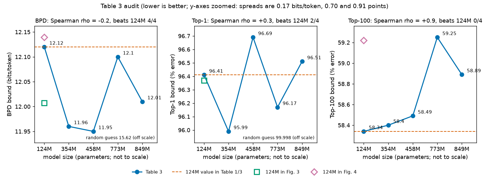
Sort each column from best (lowest) to worst:

• BPD: 458M < 354M < 849M < 773M < 124M. The step pattern as size grows is down, down, up, down. Not monotone. Spearman \(\rho = -0.2\).
• Top-1: 354M < 773M < 124M < 849M < 458M. Steps: down, up, down, up. Not monotone. \(\rho = +0.3\) (larger tends to be slightly worse).
• Top-100: 124M < 354M < 458M < 849M < 773M. Steps: up, up, up, down. Not monotone. \(\rho = +0.9\): larger is almost consistently worse.

How many of the four larger models beat the 124M model? (A "point" below is a percentage point of error: 96.41 % minus 95.99 % is 0.42 points.)

Metric	Larger models beating 124M	Differences from 124M	Spread (max − min)
BPD	4 of 4	−0.16, −0.17, −0.02, −0.11 bits/token	0.17 bits/token
Top-1	2 of 4	−0.42, +0.28, −0.24, +0.10 points	0.70 points
Top-100	0 of 4	+0.06, +0.15, +0.91, +0.55 points	0.91 points

What does this support? The paper's literal sentence in §6.4 is correct: in Table 3, the 124M model has the worst BPD bound. The caption's statement that all larger BPD bounds are tighter than the GPT-2-small bound is also correct against Table 1. What it does not support is "the bound improves as the model grows": among the four larger models, the bound goes down, up and down again, and \(\rho = -0.2\) is weak. If the five BPD values were assigned to the five sizes in a random order, a correlation of \(-0.2\) or lower would happen with probability 0.392. For top-1 the direction is mixed, and for top-100 it is opposite to the claim: a correlation of \(+0.9\) or higher happens with probability 0.042 under random assignment.

How to read these p-values

MY EXPLANATION With five points and three metrics chosen after looking at the table, a p-value of 0.042 is a description, not a discovery. It says the top-100 ordering is about as "trend-like" as five numbers can be, in the wrong direction for the paper's claim. It does not prove that size hurts top-100 bounds.

(b) How big is a difference of 0.17 bits per token?

To judge the BPD spread we need a yardstick. Four candidates, all printed by the script:

1. The subsampling term of Eq. (3). At \(\alpha = 0.25\) the loss interval has width \(\Delta = 17.202\) bits (Chapter 16), and the term \(\Delta\sqrt{\ln(1/((1-s)\delta))/(2n)}\) equals 0.211 bits/token (with \(\delta = 0.05\) and \(m = 8{,}009{,}762\) SOURCE: authors' code / nanoGPT, \(n = 10{,}000\)). It is the same for every model, so it shifts all bounds equally and cannot reorder them.
2. The random wobble of the subsample average \(\hat{\hat R}\) (the standard error). It is \(\sigma/\sqrt n\), where \(\sigma\) is the standard deviation of the per-document BPD across documents. The paper does not report \(\sigma\). Assuming \(\sigma\) = 0.5, 1 or 2 bits/token gives 0.005, 0.010 or 0.020 bits/token. Even the worst case allowed by the interval (\(\sigma \le \Delta/2 = 8.60\)) gives 0.086. Under plausible \(\sigma\), this source of noise is too small to explain the Table 3 differences.
3. The same architecture reported elsewhere in the paper. The 124M GPT-2-small shape appears three times: 12.12 in Table 1, 12.007 at the right end of Figure 3's BPD line, and 12.139 for the "regular" bar of Figure 4. These span a range of 0.132 bits/token, nearly the whole Table 3 spread of 0.17. If Figure 3's 12.007 is taken as the 124M baseline, only 2 of the 4 larger models beat it.
4. The tuning handicap. The larger models had 4 training runs; the 124M model had 72. How much does picking the best of 4 rather than the best of about 12 cost? Figure 3's dots let us estimate this (deeper block below): at each of its eight sizes there are 10–12 trained models. The expected best of 4 randomly chosen ones is worse than the best of all by 0.086 bits/token on average (range 0.051 to 0.132).

The fair summary is two-sided. The tuning handicap works against the larger models, so their 4-of-4 win on BPD is, if anything, understated; this supports the authors' limitation note. But the reported values for one and the same architecture (yardstick 3; different, unidentified runs or settings) differ by about as much as the effect, and there are no repeated seeds. The data are consistent with "larger models are at least as good on BPD" and do not establish "better and better with size". For top-1 and top-100 the data do not support the claim at all.

Paper erratum E24: Figure 3's GPT-2-small point disagrees with Table 1

PAPER Fig. 3, p. 8; Table 1, p. 6 Read exactly from the PDF's vector data, Figure 3's best BPD bound at the GPT-2-small shape (124.75M counted parameters) is 12.007, and at 7.57M parameters 11.962. Table 1 reports 12.12 as the best GPT-2-small bound. The paper does not explain the difference. It matters here because the "beats 124M" count for Table 3 drops from 4 of 4 to 2 of 4 if 12.007 is used.

(c) Figure 3: the best-bound lines

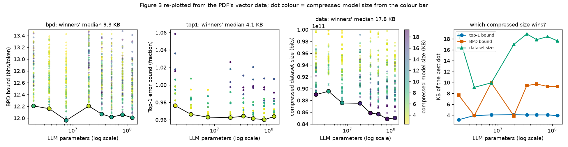
The best-bound lines, read exactly from the PDF (the project's fig_extract.py), over parameter counts from 1.90M to 124.75M:

• BPD bound: 12.207, 12.160, 11.962, 12.205, 12.068, 12.019, 12.057, 12.007 bits/token. Five of seven steps go down. \(\rho = -0.571\). The minimum is at 7.57M parameters, not at the largest model. The last value is 0.9836 times the first: a small gain across the whole range from 1.90M to 124.75M parameters.
• Top-1 bound: 0.9761, 0.9662, 0.9630, 0.9625, 0.9641, 0.9614, 0.9600, 0.9637. Five of seven steps down, \(\rho = -0.643\), minimum at 82.34M. The best top-1 bound improves slightly with parameters.
• Compressed dataset size: \(8.899 \times 10^{10}\) down to \(8.503 \times 10^{10}\); five of seven steps down, \(\rho = -0.952\), minimum at 82.34M.

So within Figure 3, all three lines tend downward with size, the dataset-size line most consistently. This is the strongest support in the paper for "bigger is better". It covers models up to GPT-2-small only, and the BPD line moves by tenths of a bit, the same size as the discrepancies of (b).

The caption puzzle (erratum E23). The caption says classification bounds "favour smaller models". The top-1 line just shown goes down as parameters grow, so the caption is wrong if "smaller" means fewer parameters. The colours offer another reading. We mapped each dot's fill colour to KB using the colour-bar image embedded in the PDF (the bar spans 2.37 to 19.32 KB; the worst colour mismatch is 0.0029 on a 0-to-1 scale). The compressed size of the winning dot at each parameter count is:

Panel	KB of best dot at the 8 sizes	Median
Top-1 bound	3.17, 3.94, 4.05, 4.11, 4.05, 4.05, 4.05, 3.94	4.05 KB
BPD bound	7.68, 3.94, 9.94, 3.89, 9.44, 9.72, 9.28, 9.28	9.28 KB
Dataset size	18.74, 9.11, 9.94, 16.98, 18.91, 17.86, 18.41, 17.64	17.75 KB

Top-1 bounds favour small compressed models, dataset size favours large compressed models, and BPD sits in between. Under this reading the caption is right for the typical (median) winner, though not at every size: at the fourth size the BPD winner (3.89 KB) is slightly smaller than the top-1 winner (4.11 KB). The table also shows the per-metric selection of erratum E66 directly: at 7 of the 8 sizes the top-1 winner and the BPD winner have different compressed sizes, so they are different trained models. Why the three panels prefer different sizes is explained by the "price of one extra KB" (deeper block below): at the typical winning sizes (with \(\delta = 0.05\) and \(m = 8{,}009{,}762\) SOURCE: authors' code / nanoGPT), one more KB costs 0.0518 bits/token on the BPD bound, 0.442 points on the top-1 bound, but only \(9.07 \times 10^{-7}\) bits/token on the dataset size.

Paper erratum E23: which models are 'smaller'?

PAPER Fig. 3 caption, p. 8 "Classification error bounds consistently favor smaller models" contradicts the middle panel if "smaller" means fewer LLM parameters (its best line falls from 0.9761 to 0.9637). It is consistent if "smaller" means smaller compressed size (the winning top-1 dots have a median of 4.05 KB, versus 9.28 KB for BPD and 17.75 KB for dataset size). The caption should say "smaller compressed size".

A note on "simpler representations". §7.1 says larger models find simpler representations. The winning BPD dots do not get smaller in KB as parameters grow (the BPD row of the table above jumps between 3.89 and 9.94 KB with no trend). What improves with size is the combination of fit and compressed size, not the compressed size alone.

A structural fact we can check. Each parameter count has 96 dots, made of 10 to 12 distinct colours, and in 84 of 90 colours the 8 top-1 dots coincide exactly. This fits "about 12 trained models, each scored at 8 values of \(\alpha\)": the top-1 bound does not depend on \(\alpha\), because mixing with the uniform distribution never changes which token is most likely (Chapter 16 proves this). The 6 exceptions are colour collisions between two models of nearly equal size.

(d) The compressed dataset size is essentially training loss

The panel's axis has no unit (erratum E26). Read as bits and divided by OpenWebText's 9,035,582,198 training tokens [SOURCE: nanoGPT prepare.py], the best line runs from 9.849 bits/token (1.90M parameters) to 9.410 bits/token (124.75M), a change of −4.45 %. For comparison, coding every token uniformly would cost \(1.411 \times 10^{11}\) bits, i.e. 15.617 bits/token.

How much of the total is the model? At 124.75M the winning dot is a 17.64 KB model, i.e. 144,539 bits: a share of \(1.70 \times 10^{-6}\) of the total. So the panel measures, up to a relative correction of about one part in a million, the average training loss of the smoothed model times the number of tokens. It confirms that larger models fit the training data better, a fact nobody disputes. It says almost nothing about the cost of the model.

Two further observations:

• The same model at its 8 values of \(\alpha\) gives dataset sizes from \(8.503 \times 10^{10}\) to \(8.900 \times 10^{10}\) bits, a 4.68 % range. So the data were coded with the smoothed model \(p_h\), not the raw model; the paper does not say so.
• 9.410 bits/token is well below the smoothed training BPD of the Table 1 model, 10.5945, that ch25_tables_audit.py reads from Figure 1. A different model, or a token-weighted rather than document-weighted average (erratum E28), could explain this. The paper does not say whether the panel counts all 9.04 billion tokens or extrapolates from the 10,000-document subsample.

Paper errata E26 and E71: the dataset-size axis has no unit, and what is coded is not stated

PAPER Fig. 3, right panel, p. 8 The axis reads about \(0.85 \times 10^{11}\) with no unit. Bits is the only reading that gives a sensible per-token value (9.4 bits/token). An addendum is logged as new: the panel also does not say that the data part uses the smoothed model (its values vary by 4.68 % across \(\alpha\) for one model), nor whether the data part covers all training tokens.

(e) Figure 4: does broken word order hurt generalization?

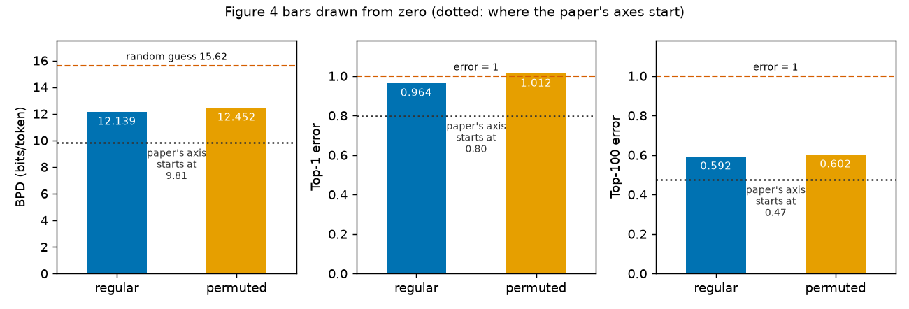
Exact bar heights, read from the PDF:

Metric	Regular	Permuted	Difference	Paper's axis starts at	True increase	Increase as drawn
BPD (bits/token)	12.1394	12.4520	+0.3126	9.806	+2.6 %	+13.4 %
Top-1 error	0.9636	1.0122	+0.0487	0.797	+5.1 %	+29.2 %
Top-100 error	0.5922	0.6022	+0.0100	0.474	+1.7 %	+8.5 %

The paper's y-axes are truncated: a truncated axis starts well above zero, so a bar's visible length is only the part above that starting value. "As drawn" is the ratio of these visible lengths. Truncation makes each difference look several times larger than it is.

The permuted top-1 bound exceeds 1: it certifies nothing, as the paper itself says. The direction (permuted is worse) holds for all three metrics. That much is supported.

The interpretation is a different matter. A bound has two parts: the measured loss \(\hat{\hat R}\) and the complexity penalty, which grows with the compressed size \(C\). The paper reports only the sum. Two extreme stories fit the bars:

• All of the rise is measured loss. Shuffled text is harder to predict. Even a perfect learner cannot predict the next word of a shuffled sentence as well as the next word of a real sentence. Then the bound rose because the task got harder, and generalization (the gap between true and measured loss) did not get worse.
• All of the rise is complexity. Then the permuted model's compressed size would have to be larger by 6.8 KB (taking 9.28 KB, the typical winning size, at \(\alpha = 0.25\); \(\delta\) and \(m\) as in (b)) for BPD, or by 17.1 KB over 4.05 KB for top-1 (more than four times the original size). Possible, but the paper gives no sign of it.

Moreover, if the bounds were evaluated on permuted documents (the text says the perturbed data are used to "train the model and evaluate the bounds"), the two bars bound the risk on two different populations: real text and shuffled text. A higher number for a harder population is not evidence of weaker generalization. The paper's claim that structure helps generalization may be true, but Figure 4 cannot separate it from "shuffled text is harder".

Paper errata E30 and E39: Figure 4's axes and its regular bars

PAPER Fig. 4, p. 9 (E30) The y-axes start at 9.806, 0.797 and 0.474, not at zero, which inflates the visible differences (true increases +2.6 %, +5.1 %, +1.7 %; drawn +13.4 %, +29.2 %, +8.5 %). (E39) The regular bars (12.139 bits/token, 96.36 % and 59.22 %) differ from Table 1's best GPT-2-small bounds (12.12, 96.41 % and 58.34 %), so the figure shows a different, unidentified run.

(erratum E70) MY EXPLANATION §7.2 also does not identify the model size, compressed sizes or \(\alpha\) of the two runs, does not report the measured loss and the complexity term separately, and does not say explicitly whether the permuted model's bound is evaluated on permuted documents (its wording suggests so). Without these, the bars cannot distinguish "worse generalization" from "harder data".

(f) Table 5: pretraining versus the majority-class baseline

Class balance of the GLUE training splits SOURCE: Hugging Face datasets-server statistics for nyu-mll/glue:

Task	Training examples	Majority class	Majority-class error	1-bit constant classifier, Eq. (1) bound	Pretrained bound	Random-init bound
QQP	363,846	not duplicate (229,468)	36.93 %	37.16 %	35.27 %	71.72 %
CoLA	8,551	acceptable (6,023)	29.56 %	31.03 %	38.89 %	53.42 %

The "constant classifier" column certifies the lazy rule with Eq. (1), \(\delta = 0.05\) SOURCE: authors' code, and a prior of \(1/2\) on each of the two constant answers (deeper block below).

What the data support:

• Pretraining helps, by a lot. On both tasks the pretrained bound is far below the random-init bound (35.27 % vs 71.72 %; 38.89 % vs 53.42 %). This is the paper's main point and it holds.
• QQP: the pretrained bound beats the majority-class error by 1.66 points and the certified constant classifier by 1.89 points. A real but modest certificate.

What they do not support:

• CoLA: the pretrained bound is 9.33 points worse than always answering "acceptable", and 7.86 points worse than the certified constant classifier. "Non-vacuous" against a 50 % coin flip, it is vacuous against the right baseline.
• Random init: both bounds exceed 50 %, so they are vacuous even by the paper's own coin-flip standard, although the text calls Table 5 "non-vacuous".

Why is CoLA so hard to certify? It has only 8,551 training sentences. Under our assumptions (Eq. 1, 0-1 loss, this \(m\), \(\delta = 0.05\)), a bound of 38.89 % would allow at most 3,704 bits (0.45 KB, i.e. 0.123 bits per subspace coordinate at \(d = 30{,}000\)) of compressed size even if the model made no training errors. For QQP the same budget is 130,559 bits (15.94 KB, 4.352 bits per coordinate). A small dataset leaves almost no room to pay for a model. That the reported CoLA bound fits into such a tiny budget is surprising, and the paper does not give enough detail (equation, \(m\), compressed sizes) to check it.

Paper erratum E22: Table 5's 'non-vacuous accuracy bounds'

PAPER App. D, p. 16 The entries are error bounds, not accuracy bounds. The random-init entries (71.72 % and 53.42 %) exceed the paper's own 50 % baseline, so they are vacuous. With class imbalance, a constant classifier errs 36.93 % (QQP) and 29.56 % (CoLA) of the time, so the pretrained CoLA bound (38.89 %) is worse than always answering "acceptable". The same pattern (captions calling every entry non-vacuous) appears in Tables 1 and 4 (erratum E65).

Paper erratum E69: Table 5's bound setting is not stated

PAPER App. D, p. 16 App. D gives the fine-tuning recipe but not the bound recipe: which equation (Eq. 1 or the subsampled Eq. 3), which loss, which data split and \(m\), which \(\delta\), the compressed sizes, or whether hyperparameter bits were paid. MY EXPLANATION Under Eq. (1) with \(m\) = GLUE training-set size and \(\delta = 0.05\), the CoLA bound of 38.89 % would require a compressed fine-tuned state of at most 3,704 bits even at zero training error. Without the setting, Table 5 cannot be reproduced.

(g) Tables 6–7: what a SubLoRA-pretrained model writes

Simple statistics of the two tables (computed from the paper's text; the texts are not reproduced):

Statistic	Table 6 (ordinary GPT-2)	Table 7 (SubLoRA)
Words	409	543
Share of the word "the"	9.0 %	22.1 %
Immediate word repeats ("the the") per 100 words	0.00	6.45
Punctuation marks per 100 characters	2.7	6.1
Share of 30 common function words	34.5 %	64.5 %

The SubLoRA text overuses the most frequent words and punctuation, the signature of a model that has learned mainly which tokens are common, not how they combine. This matches the validation loss of the SubLoRA model in Table 2, assuming the sampled model is that one or a similar one (the paper does not say; erratum E68). PAPER Table 2, p. 7 The SubLoRA model has validation BPD 10.53 and the ordinary model 4.35. MY EXPLANATION As perplexities (Chapter 6) these are \(2^{10.53} = 1{,}479\) and \(2^{4.35} = 20.4\) (also printed by ch25_tables_audit.py): at each step the SubLoRA model is as uncertain as a uniform choice among about 1,479 tokens, the ordinary model as among about 20.

This is not a criticism of the bound, which correctly certifies a weak model. It is a reminder of what is certified: the non-vacuous bounds of Tables 1 and 3 belong to models of this quality (the paper says so itself in §8; erratum E68 notes that the sampled models are not identified).

(h) Scorecard: what the data support

Two remarks of fairness first. The §6.4 text and the Table 3 caption make their size claims about BPD only; the top-k rows below test the broader wording of the abstract and §7.1 ("bounds improve with model size"). And the contributions list's stronger claim, that the results disprove "larger LLMs merely regurgitate", goes beyond what any bound here can show: the bounds concern heavily compressed SubLoRA models, not ordinary large LLMs, and a smaller upper bound on error is not a measurement of how much a model memorizes.

Claim	Verdict	Evidence
Larger models (354M–849M) have non-vacuous BPD bounds	Supported	All Table 3 BPD bounds lie between 11.95 and 12.12, below 15.62
Every larger model's BPD bound beats Table 1's 124M bound	Supported, fragile	4 of 4; only 2 of 4 against Figure 3's 12.007
BPD bound improves steadily with size	Not supported	Non-monotone; \(\rho = -0.2\); spread 0.17 ≈ same-architecture differences
Top-k bounds improve with size	Not supported	Top-1 2 of 4, \(\rho = +0.3\); top-100 0 of 4, \(\rho = +0.9\)
Within Figure 3 (≤ 124.75M), bounds and dataset size fall with size	Mostly supported	5 of 7 steps down on each line; small effects on BPD
"Larger models are more compressible"	Only as total code length	The model is \(1.70 \times 10^{-6}\) of the dataset size; winning \(C(h)\) does not shrink
This disproves "larger LLMs merely regurgitate"	Overreach	Bounds are for compressed SubLoRA models; a bound is not a memorization measurement
Broken word order gives worse bounds	Supported as a fact about bounds	All three bars rise; no seeds
Broken word order hurts generalization	Not established	No split into loss and complexity; different populations
Pretraining gives much better bounds	Supported	35.27 vs 71.72; 38.89 vs 53.42
Table 5 bounds are non-vacuous	Only pretrained QQP	CoLA worse than majority class; random-init above 50 %

Going deeper

This hub collects the derivations behind the audits above. Everything here is MY EXPLANATION unless tagged.

Going deeper: Spearman's rho and the exact permutation test

Definition. Given \(n\) paired values \((a_i, b_i)\) with no ties, let \(r_i\) be the rank of \(a_i\) among the \(a\)'s and \(q_i\) the rank of \(b_i\) among the \(b\)'s (1 = smallest). Spearman's \(\rho\) is the ordinary (Pearson) correlation of the ranks:

\[ \rho = \frac{\frac1n \sum_i r_i q_i - \bar r\, \bar q}{\operatorname{sd}(r)\,\operatorname{sd}(q)} . \]

Closed form. Both rank lists are the numbers \(1, \dots, n\) in some order. Their mean is \(\bar r = \bar q = (n+1)/2\). Their mean square is \(\frac1n\sum_{k=1}^n k^2 = (n+1)(2n+1)/6\). So their variance is

\[ \frac{(n+1)(2n+1)}{6} - \frac{(n+1)^2}{4} = \frac{(n+1)\big(2(2n+1) - 3(n+1)\big)}{12} = \frac{(n+1)(n-1)}{12} = \frac{n^2-1}{12}. \]

Let \(d_i = r_i - q_i\). Expanding \(\sum_i d_i^2 = \sum_i r_i^2 + \sum_i q_i^2 - 2\sum_i r_i q_i\) and using \(\sum r_i^2 = \sum q_i^2\) gives \(\frac1n\sum_i r_i q_i = \frac{(n+1)(2n+1)}{6} - \frac{1}{2n}\sum_i d_i^2\). Subtracting \(\bar r \bar q = (n+1)^2/4\) leaves \(\frac{n^2-1}{12} - \frac{1}{2n}\sum_i d_i^2\). Dividing by the variance \(\frac{n^2-1}{12}\):

\[ \rho = 1 - \frac{6 \sum_i d_i^2}{n(n^2-1)} . \]

Table 3, BPD, by hand. Sizes in order 124, 354, 458, 773, 849M have ranks 1–5. The BPD values 12.12, 11.96, 11.95, 12.10, 12.01 have ranks 5, 2, 1, 4, 3. The differences are \(-4, 0, 2, 0, 2\), so \(\sum d_i^2 = 24\) and \(\rho = 1 - 6 \cdot 24 / (5 \cdot 24) = 1 - 1.2 = -0.2\), matching the script. For top-1 the ranks are 3, 1, 5, 2, 4, the differences \(-2, 1, -2, 2, 1\), \(\sum d_i^2 = 14\) and \(\rho = 1 - 84/120 = +0.3\).

Because \(\rho\) depends only on ranks, using size or the logarithm of size gives the same value.

The permutation test. Keep the five bound values fixed and imagine assigning them to the five sizes in a uniformly random order: \(5! = 120\) equally likely orders. For each, compute \(\rho\). The exact one-sided p-value is the fraction of orders whose \(\rho\) is at least as extreme as the observed one. The script enumerates all 120. What is random: only the hypothetical assignment. What is fixed: the values and the sizes. This test does not model how the values were produced (training noise, sweep sizes); it only asks whether the observed ordering is unusual among all orderings. With \(n = 5\) the smallest achievable one-sided p-value is \(1/120\) (perfect order), so even a perfect trend would be weak evidence.

Going deeper: the standard error of the subsample average, and the worst case

Setting. The trained model \(h\) is fixed. The \(m\) training documents are fixed. Let \(y_j = R(h, X_j)\) be the BPD of document \(j\) (bits/token), with mean \(\hat R(h)\) and population variance \(\sigma^2 = \frac1m \sum_j (y_j - \hat R)^2\) over the \(m\) documents. The subsample picks indices \(J_1, \dots, J_n\) at random; this is the only randomness. Write \(\hat{\hat R} = \frac1n\sum_{i=1}^n y_{J_i}\).

With replacement. The draws \(Y_i = y_{J_i}\) are independent, each with mean \(\hat R\) and variance \(\sigma^2\). Variances of independent variables add, and scaling by \(1/n\) scales variance by \(1/n^2\):

\[ \operatorname{Var}\big(\hat{\hat R}\big) = \frac{1}{n^2}\sum_{i=1}^n \operatorname{Var}(Y_i) = \frac{\sigma^2}{n}, \qquad \text{standard error} = \frac{\sigma}{\sqrt n}. \]

Without replacement. The draws are no longer independent. By symmetry every pair of distinct draws has the same covariance \(c\). Then \(\operatorname{Var}(\sum_{i=1}^n Y_i) = n\sigma^2 + n(n-1)c\). If we draw all \(n = m\) documents, the sum is the fixed total, whose variance is 0, so \(m\sigma^2 + m(m-1)c = 0\), i.e. \(c = -\sigma^2/(m-1)\). Substituting back:

\[ \operatorname{Var}\big(\hat{\hat R}\big) = \frac{\sigma^2}{n}\left(1 - \frac{n-1}{m-1}\right) = \frac{\sigma^2}{n}\cdot\frac{m-n}{m-1} . \]

With \(n = 10{,}000\) and \(m = 8{,}009{,}762\) SOURCE: nanoGPT the factor is 0.99875, so \(\sigma/\sqrt n\) is the right size.

Worst case (Popoviciu's inequality). If every \(y_j\) lies in an interval \([a, b]\), then \(\sigma \le (b-a)/2\). Proof: for any constant \(c\), \(\frac1m\sum_j (y_j - c)^2 = \sigma^2 + (\hat R - c)^2 \ge \sigma^2\) (expand the square around \(\hat R\); the cross term averages to zero). Choose \(c = (a+b)/2\); then \(|y_j - c| \le (b-a)/2\) for every \(j\), so \(\sigma^2 \le ((b-a)/2)^2\). For BPD at \(\alpha = 0.25\) the interval width is \(\Delta = 17.202\) bits, so \(\sigma \le 8.60\) and the standard error is at most 0.086 bits/token. Real per-document BPD values cluster far more tightly than a two-point distribution at the interval's ends, which is why we also print the assumed \(\sigma\) = 0.5–2 cases.

Why the subsampling term of Eq. (3) does not reorder models. The term \(\Delta\sqrt{\ln(1/((1-s)\delta))/(2n)}\) depends only on \(\Delta\), \(n\), \(m\) (through \(s\)) and \(\delta\), not on the model. All Table 3 bounds (at the same \(\alpha\)) carry the same 0.211 bits/token. What can reorder models is the realized subsample average, whose wobble is the standard error above, and the training run itself.

Going deeper: the best-of-k effect of a larger sweep

Suppose a size has \(N\) trained models with (best-\(\alpha\)) bounds sorted as \(v_{(1)} \le v_{(2)} \le \dots \le v_{(N)}\). If only \(k\) of them had been trained, chosen at random, what would the best one be on average?

The minimum of the chosen \(k\) equals \(v_{(i)}\) exactly when model \(i\) is chosen and the other \(k-1\) come from the \(N - i\) models ranked above it. There are \(\binom{N-i}{k-1}\) such choices out of \(\binom{N}{k}\), so

\[ \mathbb E\big[\min \text{ of } k\big] = \sum_{i=1}^{N} v_{(i)}\,\frac{\binom{N-i}{k-1}}{\binom{N}{k}} . \]

The script computes the same quantity by averaging the minimum over all \(\binom Nk\) subsets. With \(k = 4\) and Figure 3's 10–12 models per size, the expected best of 4 is above the best of all by 0.051 to 0.132 bits/token (mean 0.086).

What this means and does not mean. The randomness is in which \(k\) settings are tried; the trained models are fixed. It shows that "more tries" alone lowers the reported best bound by a few hundredths to a tenth of a bit. This is a stand-in: the larger models' 4 settings were not chosen at random (they reuse the learning rate and rank that worked for 124M), and the 124M sweep had 72 runs, not 12, so its advantage could be larger. Either way, the effect is of the same size as the Table 3 differences, and it favours the 124M model. This supports the authors' limitation note.

There is also a statistical side. Selecting the best of many runs is allowed in the bound only because the hyperparameters are paid for in the prior (Chapter 24): 576 settings cost \(\log_2 576\) bits (under 10 bits), a negligible amount next to a \(C(h)\) of tens of thousands of bits (Figure 3's winners are 3–19 KB). So the sweep does not invalidate any bound; it only makes bounds from differently sized sweeps unequal competitors.

Going deeper: why the three Figure 3 panels prefer different compressed sizes

Each panel minimizes "fit + price of the model", with a different price.

Bounds. For a model of compressed size \(C\) bits, Eq. (3) adds \(\Delta \cdot t_m(C) + \Delta \cdot t_n\) to the measured loss, where

\[ t_m(C) = \sqrt{\frac{C\ln 2 + 2\ln C + \ln\frac{1}{s\delta}}{2m}}, \qquad t_n = \sqrt{\frac{\ln\frac{1}{(1-s)\delta}}{2n}} . \]

Only \(t_m\) depends on \(C\). Its derivative is

\[ \frac{d t_m}{dC} = \frac{\ln 2 + 2/C}{2\sqrt{2m}\,\sqrt{C\ln 2 + 2\ln C + \ln\frac{1}{s\delta}}} \approx \frac{\ln 2}{2\sqrt{2m\, C \ln 2}} , \]

which falls like \(1/\sqrt C\). Multiplying by \(\Delta\) and by 8,192 bits per KB gives the price of one extra KB. The script evaluates the exact finite difference: at 9.28 KB with \(\Delta = 17.202\) bits (BPD, \(\alpha = 0.25\)) it is 0.0518 bits/token; at 4.05 KB with \(\Delta = 1\) (top-1) it is 0.442 percentage points (\(\delta = 0.05\), \(m = 8{,}009{,}762\) SOURCE: authors' code / nanoGPT).

Dataset size. Here the model's bits are added once to a total of about \(8.5 \times 10^{10}\) bits. One extra KB adds 8,192 bits, i.e. \(8{,}192 / 9{,}035{,}582{,}198 = 9.07 \times 10^{-7}\) bits per token. Model size is almost free, so the largest compressed models (best fit) win.

Top-1 versus BPD. A bigger compressed model must buy enough improvement in measured loss to pay its price. The top-1 bounds barely move with capacity (the best line of Figure 3 stays between 0.9600 and 0.9761 across all eight sizes), which suggests that measured top-1 error improves little when the model grows. Extra KB then rarely pay off: small compressed models win. Measured BPD improves more with capacity, so BPD settles at intermediate sizes. This is the mechanism behind the caption's sentence, under the "compressed size" reading.

Going deeper: the compressed dataset size as a two-part code

MY EXPLANATION A receiver who knows the architecture and the coding rules can rebuild the training set from two messages: the model \(h\) (\(C(h)\) bits, from Chapter 24's pipeline), then the tokens coded by arithmetic coding under \(p_h\). Chapter 22 shows the second message costs at most the total surprisal \(\sum -\log_2 p_h(x_i \mid x_{<i})\) plus 2 bits. So the panel is an upper bound (up to a constant for the decoder program) on the Kolmogorov complexity of the training set (Chapter 13).

Units. Total bits divided by tokens gives bits/token. With \(N_{\text{tok}} = 9{,}035{,}582{,}198\) SOURCE: nanoGPT, the 124.75M point is 9.410 bits/token, of which the model contributes \(1.70 \times 10^{-6}\) of the total. Note this is a token-weighted average (every token counts once), while the bound's \(\hat R\) is a document-weighted average of per-document BPD (Chapter 15). The two coincide only if all documents have equal length or equal BPD.

Why it is not a generalization statement. The dataset size is computed on the training data only. A model that memorized every document perfectly would need few data bits but a huge \(C(h)\); the sum penalizes that. However, at these sizes \(C(h)\) is a millionth of the total, so in practice the panel ranks models by training loss. It shows that larger SubLoRA models fit better; whether they generalize better is what the bound panels measure, and those move far less.

Going deeper: separating loss from complexity in Figure 4

Write the BPD bound of a model at smoothing weight \(\alpha\) as

\[ B = \hat{\hat R} + \Delta(\alpha)\,\big(t_m(C) + t_n\big), \]

with \(t_m\), \(t_n\) as in the previous block. For the regular (r) and permuted (p) models at the same \(\alpha\),

\[ B_p - B_r = \big(\hat{\hat R}_p - \hat{\hat R}_r\big) + \Delta(\alpha)\big(t_m(C_p) - t_m(C_r)\big). \]

The paper reports \(B_p - B_r = 0.3126\) bits/token but neither term on the right. If the measured losses were equal, the second term would have to supply all of it; solving \(\Delta(\alpha)(t_m(C_r + x) - t_m(C_r)) = 0.3126\) with \(C_r\) = 9.28 KB and \(\alpha = 0.25\) gives \(x = 6.8\) KB. The same computation for top-1 (\(\Delta = 1\), \(C_r\) = 4.05 KB, rise 0.0487) gives 17.1 KB.

Why the measured loss should rise. Within a shuffled sequence, the next token is a random one of the tokens not yet shown. Even a model that knew the document's full word list would be uncertain which comes next, while in real text grammar narrows the choice. So the best achievable loss on shuffled text is higher. This is a plausibility argument; the paper does not measure achievable loss on shuffled text.

What would settle it. Report \(\hat{\hat R}\) and \(C\) for both models (with seeds), and, for a cleaner comparison, the gap between validation loss and training loss under each data distribution.

Going deeper: certifying the constant classifier, and the CoLA budget

The lazy hypothesis class. Take the two classifiers "always answer class A" and "always answer class B", with prior \(P = 1/2\) each, so \(\ln(1/P(h)) = \ln 2\) nats. The loss is the 0-1 loss (interval width \(\Delta = 1\)). By Eq. (1) (Chapter 11), with probability at least \(1-\delta\) over the random draw of the \(m\) training examples, both classifiers satisfy

\[ R(h) \le \hat R(h) + \sqrt{\frac{\ln 2 + \ln(1/\delta)}{2m}} . \]

For CoLA, "always acceptable" has \(\hat R = 2{,}528/8{,}551 = 29.56\,\%\) SOURCE: HF datasets-server and \(m = 8{,}551\); with \(\delta = 0.05\) SOURCE: authors' code the bound is 31.03 %. For QQP, \(\hat R = 36.93\,\%\), \(m = 363{,}846\), and the bound is 37.16 %. These are honest, certified baselines in exactly the paper's framework, and a learned model must beat them to show that it learned something certifiable.

The CoLA budget. For a learned model with compressed size \(C\) bits, the paper's prior gives \(\ln(1/P(h)) \le C\ln 2 + 2\ln C\) (Chapter 14). Setting the measured error to zero (the most favourable case) and asking for a bound of at most 38.89 %:

\[ \sqrt{\frac{C\ln 2 + 2\ln C + \ln(1/\delta)}{2 \cdot 8{,}551}} \le 0.3889 . \]

Bisection gives \(C \le 3{,}704\) bits. Any training error lowers this budget further. With \(d = 30{,}000\) subspace coordinates, that is at most 0.123 bits per coordinate. Arithmetic coding can reach such rates only if almost all coordinates fall into one quantization level. Under these assumptions the reported number is possible but surprising, and the missing setting (new erratum above) prevents a check.

Common misconceptions

• Misconception: Table 3 shows that the bound improves as models grow. — Actually: the BPD bounds go 12.12, 11.96, 11.95, 12.10, 12.01 with size: lower than 124M for every larger model, but not monotone, with a rank correlation of only −0.2. Top-1 is mixed and top-100 gets worse for every larger model.
• Misconception: a difference of 0.17 bits/token between single runs is a reliable ranking. — Actually: the paper itself reports the 124M shape at 12.12, 12.007 and 12.139 in different places (a range of 0.132), and gives no seeds or error bars.
• Misconception: the falling "compressed dataset size" shows that larger models need fewer bits to describe themselves. — Actually: the model is \(1.70 \times 10^{-6}\) of the total; the panel is training loss times tokens. The winning models' compressed sizes do not shrink with parameter count.
• Misconception: Figure 4 shows that shuffled text makes models generalize worse. — Actually: it shows a higher bound, which may come entirely from shuffled text being harder to predict. The paper does not split the bound into measured loss and complexity.
• Misconception: an error bound below 50 % on a two-class task is non-vacuous. — Actually: the right baseline is the majority class. On CoLA, always answering "acceptable" errs 29.56 % of the time, so the 38.89 % bound certifies less than the laziest rule.
• Misconception: the larger models' smaller sweep is a flaw that inflates the paper's size claim. — Actually: it works against the claim: with more tuning the larger models would probably do better (the best-of-k estimate is about 0.09 bits/token). This strengthens "at least as good", not "steadily better".

Self-test

Q1. Compute Spearman's \(\rho\) between model size and the Table 3 top-100 bounds (58.34, 58.4, 58.49, 59.25, 58.89 for 124M to 849M). What does its sign say about the paper's claim?

Answer

Ranks of the bounds (1 = smallest) in size order: 58.34 → 1, 58.4 → 2, 58.49 → 3, 59.25 → 5, 58.89 → 4. The size ranks are 1, 2, 3, 4, 5, so the differences are 0, 0, 0, −1, 1 and \(\sum d_i^2 = 2\). Then \(\rho = 1 - 6 \cdot 2/(5 \cdot 24) = 1 - 0.1 = +0.9\), as the script prints. For a lower-is-better bound, a positive \(\rho\) means larger models have worse top-100 bounds, the opposite of "larger models have better bounds". With five points it is a description, not proof.

Q2. Why does the right panel of Figure 3 favour the largest compressed models, while the top-1 panel favours the smallest?

Answer

In the dataset-size panel, the model's bits are added once to about \(8.5 \times 10^{10}\) bits of data, so one more KB costs only \(9.07 \times 10^{-7}\) bits per token; any improvement in fit is worth it, so the best-fitting (largest) compressed models win. In a bound, the model's bits enter through \(\sqrt{C\ln 2/(2m)}\) multiplied by the loss width, which costs 0.442 percentage points per extra KB for top-1 at 4.05 KB. Top-1 error barely improves with capacity, so extra KB do not pay for themselves and small compressed models win. This is the reading under which the Figure 3 caption is correct (erratum E23).

Q3. QQP's training split has 363,846 pairs, of which 229,468 are "not duplicate". Is the pretrained QQP bound of 35.27 % non-vacuous in a meaningful sense? What about the CoLA bound of 38.89 %?

Answer

The majority-class error on QQP is \(1 - 229{,}468/363{,}846 = 36.93\,\%\), and certifying the constant classifier with Eq. (1) (\(\delta = 0.05\)) gives 37.16 %. The pretrained bound 35.27 % is 1.89 points below that, so it certifies something the lazy rule cannot: meaningful, though modest. On CoLA the majority-class error is 29.56 % (certified: 31.03 %), so the 38.89 % bound is worse than always answering "acceptable". It is non-vacuous only against the 50 % coin flip the paper uses, not against the right baseline.

Code for this chapter

The script audits Table 3 (rank orders, Spearman correlations with exact permutation p-values, spreads, "beats 124M" counts), compares the spreads with four yardsticks, analyses Figure 3 from the PDF's vector data (best lines, dot colours mapped to KB, the best-of-k effect, the price of a KB, the dataset size per token), redraws Figure 4 from zero, compares Table 5 with the GLUE class balance, and computes text statistics for Tables 6–7. It reads outputs/fig_extract.json (the project's exact figure data, written by fig_extract.py) and the GLUE statistics files under sources/ext/.

Run it from the project root:

.venv/Scripts/python explainer/code/ch26_table3_audit.py

Source: ch26_table3_audit.py

"""Chapter 26 demo: scale, structure and pretraining (§6.4, §7, App. D, App. F of arXiv 2312.17173).

Claims reproduced / checked (paper values typed in from the PDF; figure data read from the PDF's vector graphics):
  [1] Table 3: is each column monotone in model size? rank order, Spearman correlation with size (exact
      permutation p-value), spread, how many larger models beat 124M (claim C6, erratum E29).
  [2] Scales to compare the Table 3 spreads with: the subsampling term of Eq. (3) at alpha = 0.25, the Monte-Carlo
      standard error of the subsampled empirical risk (ASSUMED per-document spread; worst case by Popoviciu), and
      the same-architecture discrepancies Fig. 3 / Fig. 4 vs Table 1 (E24, E39).
  [3] Sweep-size handicap (MY ANALYSIS): expected best of 4 vs best of 12 trained models, using Fig. 3's dots.
  [4] Figure 3 best-bound lines: monotonicity and Spearman correlation (claims C6, C11).
  [5] Figure 3 colours -> compressed model size (KB) via the embedded colourbar image (erratum E23); the
      12-models x 8-alpha structure of the dots.
  [6] Compressed dataset size: bits per token over OpenWebText's 9,035,582,198 tokens, model share (C12, E26).
  [7] Figure 4: bars, truncated axes, drawn vs true ratios (E30, E39); claim C10.
  [8] Table 5 vs class balance (E22): majority-class errors, a 1-bit constant classifier's Eq. (1) bound, and the
      largest compressed size Eq. (1) would allow for the pretrained bounds.
  [9] Tables 6-7 (App. F): simple text statistics (no text reproduced) and perplexities 2^10.53, 2^4.35.
Assumptions not stated in the paper (labelled in the output): delta = 0.05, m = 8,009,762 documents [SOURCE:
authors' code / nanoGPT]; 1 KB = 8192 bits (E35); V = 50,257; GLUE class counts [SOURCE: HF datasets-server].
Writes outputs/ch26_table3_audit.txt and docs/assets/fig/ch26_table3.png, ch26_fig3_replot.png, ch26_fig4_axes.png.
"""
from __future__ import annotations

import itertools
import json
import math
import re
import sys
import time
from pathlib import Path

HERE = Path(__file__).resolve().parent
sys.path.insert(0, str(HERE))

import matplotlib  # noqa: E402

matplotlib.use("Agg")
import matplotlib.pyplot as plt  # noqa: E402
import numpy as np  # noqa: E402
import pymupdf as fitz  # noqa: E402

import fig_extract as fe  # noqa: E402  (PDF-reading helpers shared with the orchestrator's extractor)
import pacbound as pb  # noqa: E402

ROOT = HERE.parent.parent
OUT = HERE / "outputs"
FIG = HERE.parent / "docs" / "assets" / "fig"
OUT.mkdir(exist_ok=True)
FIG.mkdir(parents=True, exist_ok=True)
T0 = time.time()
LINES: list[str] = []
KB_BITS = 8192  # E35


def say(s: str = "") -> None:
    LINES.append(s)


def spearman(x, y) -> float:
    rx = np.argsort(np.argsort(x)) + 1.0
    ry = np.argsort(np.argsort(y)) + 1.0
    n = len(x)
    return 1.0 - 6.0 * float(((rx - ry) ** 2).sum()) / (n * (n * n - 1))


def exact_perm_p(x, y, observed: float) -> tuple[float, float]:
    """Exact permutation p-values P(rho <= observed), P(rho >= observed) over all orderings of y."""
    rhos = [spearman(x, list(p)) for p in itertools.permutations(y)]
    lo = sum(r <= observed + 1e-12 for r in rhos) / len(rhos)
    hi = sum(r >= observed - 1e-12 for r in rhos) / len(rhos)
    return lo, hi


# ============================================================================ [1] Table 3
SIZES_M = np.array([124, 354, 458, 773, 849])                     # [PAPER §6.4, Table 3] millions of parameters
T3 = {"BPD": [12.12, 11.96, 11.95, 12.10, 12.01],                 # bits/token
      "Top-1": [96.41, 95.99, 96.69, 96.17, 96.51],               # % error
      "Top-100": [58.34, 58.4, 58.49, 59.25, 58.89]}              # % error ("58.4": E29)
say("Chapter 26 - scale, structure, pretraining audit (ch26_table3_audit.py)")
say(f"[0] delta = {pb.DELTA}, m = {pb.M_DOCS:,} docs [SOURCE: authors' code/nanoGPT]; n = {pb.N_SUB:,}; "
    f"1 KB = {KB_BITS} bits (E35); V = {pb.V_GPT2:,}")
say("[1] Table 3 [PAPER] vs size 124/354/458/773/849M (lower = better). Spearman rho with size (= with log size)")
say("  values: " + " | ".join(f"{k} " + " ".join(f"{x:g}" for x in v) for k, v in T3.items()))
res3 = {}
for name, v in T3.items():
    v = np.array(v)
    rho = spearman(SIZES_M, v)
    plo, phi = exact_perm_p(SIZES_M, list(v), rho)
    steps = np.sign(np.diff(v))
    order = "<".join(f"{SIZES_M[i]}" for i in np.argsort(v))
    beat = int((v[1:] < v[0]).sum())
    spread = v.max() - v.min()
    mono = "monotone" if (np.all(steps < 0) or np.all(steps > 0)) else "NOT monotone"
    res3[name] = (rho, beat, spread)
    say(f"  {name:7s} best->worst {order}; {mono} (steps {''.join('+' if s > 0 else '-' for s in steps)}); "
        f"rho {rho:+.1f} (exact P(rho<=obs) {plo:.3f}, P(rho>=obs) {phi:.3f})")
    unit = "bits/token" if name == "BPD" else "pct pts"
    say(f"          spread max-min {spread:.2f} {unit}; larger models beating 124M: {beat}/4; "
        f"diffs vs 124M {', '.join(f'{d:+.2f}' for d in v[1:] - v[0])}")
assert res3["BPD"][1] == 4 and res3["Top-1"][1] == 2 and res3["Top-100"][1] == 0
assert abs(res3["BPD"][0] + 0.2) < 1e-9 and abs(res3["Top-1"][0] - 0.3) < 1e-9 and abs(res3["Top-100"][0] - 0.9) < 1e-9

# ============================================================================ [2] noise scales
fj = json.loads((OUT / "fig_extract.json").read_text(encoding="utf-8"))
f3, f4 = fj["figure3"], fj["figure4"]
lo, hi, D25 = pb.smoothing_interval(0.25)
s = pb.N_SUB / (pb.N_SUB + pb.M_DOCS)
t_n_bpd = pb.hoeffding_t(pb.N_SUB, D25, math.log(1 / ((1 - s) * pb.DELTA)))
t_n_top = pb.hoeffding_t(pb.N_SUB, 1.0, math.log(1 / ((1 - s) * pb.DELTA)))
say("[2] Scales to compare with (bits/token for BPD; pct pts for top-k)")
say(f"  subsampling term Delta*sqrt(ln(1/((1-s)delta))/2n): BPD (alpha 0.25, Delta {D25:.3f}) {t_n_bpd:.3f}; "
    f"top-k (Delta 1) {100 * t_n_top:.2f} pts  [same for every model -> shifts, does not reorder]")
se_assumed = {sig: sig / math.sqrt(pb.N_SUB) for sig in (0.5, 1.0, 2.0)}
say("  Monte-Carlo s.e. of R^^ = sigma/sqrt(n), ASSUMED per-document sigma (bits/token): "
    + ", ".join(f"{k:.1f} -> {v:.3f}" for k, v in se_assumed.items())
    + f"; worst case sigma <= Delta/2 = {D25 / 2:.2f} -> {D25 / 2 / math.sqrt(pb.N_SUB):.3f}")
say(f"  top-k s.e.: ASSUMED sigma 0.05 -> {100 * 0.05 / math.sqrt(pb.N_SUB):.2f} pts; worst case sigma <= 0.5 -> "
    f"{100 * 0.5 / math.sqrt(pb.N_SUB):.2f} pts")
fig3_124_bpd = f3["bpd_bound"]["best_line"][-1]["value"]
fig3_124_top1 = f3["top1_error_bound"]["best_line"][-1]["value"]
say(f"  same 124M architecture elsewhere: BPD Table 1 12.12 vs Fig. 3 {fig3_124_bpd:.3f} (diff "
    f"{fig3_124_bpd - 12.12:+.3f}) vs Fig. 4 regular {f4['bpd']['regular']:.3f} (diff {f4['bpd']['regular'] - 12.12:+.3f})")
say(f"     top-1 Table 1 96.41 vs Fig. 3 {100 * fig3_124_top1:.2f} vs Fig. 4 {100 * f4['top1']['regular']:.2f}; "
    f"top-100 Table 1 58.34 vs Fig. 4 {100 * f4['top100']['regular']:.2f}")
three = [12.12, fig3_124_bpd, f4["bpd"]["regular"]]
fpc = (pb.M_DOCS - pb.N_SUB) / (pb.M_DOCS - 1)
say(f"     BPD range of the three 124M values {max(three) - min(three):.3f} bits/token; "
    f"without-replacement variance factor (m-n)/(m-1) = {fpc:.5f}")
bpd3 = np.array(T3["BPD"])
beat_fig3 = int((bpd3[1:] < fig3_124_bpd).sum())
say(f"  with Fig. 3's 124M value {fig3_124_bpd:.3f} as the baseline, larger models beating it (BPD): {beat_fig3}/4")
assert abs(t_n_bpd - 0.21) < 0.005 and beat_fig3 == 2

# ============================================================================ [5] colours (needed for [3])
doc = fitz.open(ROOT / "paper.pdf")
page = doc[7]
xref = page.get_images(full=True)[0][0]
pix = fitz.Pixmap(doc, xref)
if pix.colorspace is None or pix.colorspace.n != 3:
    pix = fitz.Pixmap(fitz.csRGB, pix)
cbar = np.frombuffer(pix.samples, dtype=np.uint8).reshape(pix.height, pix.width, pix.n)[:, :, :3].astype(float) / 255
cbar_col = cbar[:, cbar.shape[1] // 2, :]                       # one column, rows top -> bottom
img_rect = page.get_image_info(xrefs=True)[0]["bbox"]           # (x0, y0, x1, y1) in PDF points
ticks = []                                                       # (y of tick mark, KB label)
labels = {round((sp[1][1] + sp[1][3]) / 2, 1): float(sp[0]) for sp in fe.spans(page, 60, 200, x0=img_rect[2])
          if fe.number(sp[0]) is not None}
drw = page.get_drawings()
for d in drw:
    r = d["rect"]
    if r.x0 >= img_rect[2] - 0.5 and r.x1 < img_rect[2] + 5 and r.y1 < 200 and abs(r.y0 - r.y1) < 0.01:
        lab = min(labels, key=lambda yc: abs(yc - r.y0))
        ticks.append((r.y0, labels[lab]))
ticks.sort()
kb_axis = fe.Axis(ticks[0][0], ticks[0][1], ticks[-1][0], ticks[-1][1])
rows = cbar_col.shape[0]
row_kb = np.array([kb_axis(img_rect[1] + (i + 0.5) / rows * (img_rect[3] - img_rect[1])) for i in range(rows)])

rects = [r for r in fe.axes_rects(drw, 200) if r.width > 30][:3]
panels = {}
max_dist = 0.0
for name, r in zip(["bpd", "top1", "data"], rects):
    vx, hy = fe.gridlines(drw, r)
    xs = [v for v in vx if r.x0 - 0.5 <= v <= r.x1 + 0.5][:3]
    xa = fe.Axis(xs[0], 1e6, xs[1], 1e7, log=True)
    labs = fe.left_labels(page, r, (60, 200))
    hy_in = [h for h in hy if r.y0 - 0.5 <= h <= r.y1 + 0.5]
    pairs = [(fe.nearest_line(hy_in, cy), v) for cy, v in labs]
    mult = 1e11 if name == "data" else 1.0
    ya = fe.Axis(pairs[0][0], pairs[0][1] * mult, pairs[-1][0], pairs[-1][1] * mult)
    dots = []
    for d in drw:
        f = d.get("fill")
        if not f or fe.col(f) == (1.0, 1.0, 1.0) or d["rect"].width > 6:
            continue
        cx, cy = fe.centre(d)
        if r.x0 <= cx <= r.x1 and r.y0 <= cy <= r.y1:
            e = ((cbar_col - np.array(f)) ** 2).sum(1)
            i = int(e.argmin())
            max_dist = max(max_dist, math.sqrt(e[i]))
            dots.append((xa(cx), ya(cy), float(row_kb[i])))
    panels[name] = dots


def groups(dots):
    g: dict[float, list] = {}
    for x, v, kb in dots:
        g.setdefault(round(math.log10(x), 2), []).append((v, kb, x))
    return [sorted(g[k]) for k in sorted(g)]


G = {k: groups(v) for k, v in panels.items()}
PARAMS = [pt["params"] for pt in f3["bpd_bound"]["best_line"]]

# ============================================================================ [3] sweep-size handicap
say("[3] Sweep-size handicap [MY ANALYSIS; Fig. 3 dots as stand-in]: per size, each trained model's best-alpha BPD;")
handicaps = []
for grp in G["bpd"]:
    per_model: dict[float, float] = {}
    for v, kb, _ in grp:
        k = round(kb, 2)
        per_model[k] = min(per_model.get(k, 99.0), v)
    vals = sorted(per_model.values())
    if len(vals) >= 4:
        e4 = np.mean([min(c) for c in itertools.combinations(vals, 4)])
        handicaps.append((len(vals), e4 - vals[0], vals[-1] - vals[0]))
hc = np.array([h[1] for h in handicaps])
say(f"  models per size {[h[0] for h in handicaps]}; E[best of 4 random models] - best of all: mean {hc.mean():.3f}, "
    f"range {hc.min():.3f}..{hc.max():.3f} bits/token")
say(f"  spread of per-model best within one size (max-min): {min(h[2] for h in handicaps):.2f}..{max(h[2] for h in handicaps):.2f}"
    f" bits/token; sweeps: 124M {6 * 2 * 3 * 2} trainings x 8 alpha = {6 * 2 * 3 * 2 * 8}; larger {2 * 2} x 8 = {2 * 2 * 8} [PAPER App. E]")

# ============================================================================ [4] Fig. 3 best lines
say("[4] Figure 3 best-bound lines (exact, fig_extract.py) vs parameters 1.90M..124.75M")
for key, lab, fmt_ in (("bpd_bound", "BPD", "{:.3f}"), ("top1_error_bound", "Top-1", "{:.4f}"),
                       ("compressed_dataset_size_bits", "data", "{:.3e}")):
    v = np.array([pt["value"] for pt in f3[key]["best_line"]])
    rho = spearman(np.array(PARAMS), v)
    steps = np.sign(np.diff(v))
    imin = int(v.argmin())
    say(f"  {lab:5s} {' '.join(fmt_.format(x) for x in v)}")
    say(f"        steps {''.join('+' if t > 0 else '-' for t in steps)} ({int((steps < 0).sum())}/7 down); rho {rho:+.3f};"
        f" min at {PARAMS[imin] / 1e6:.2f}M; last/first {v[-1] / v[0]:.4f}")

# ============================================================================ [5] colour check output
say(f"[5] Fig. 3 colour -> KB (colourbar image xref {xref}, {rows} rows, {kb_axis(img_rect[3]):.2f}..{kb_axis(img_rect[1]):.2f} KB;"
    f" max colour mismatch {max_dist:.4f} of 1)")
n_models = [len({round(kb, 2) for _, kb, _ in grp}) for grp in G["bpd"]]
n_col, n_one, n_eight = 0, 0, 0     # colours; colours whose top-1 dots share one value; colours with exactly 8 dots
for grp in G["top1"]:
    for kb in {round(kb2, 2) for _, kb2, _ in grp}:
        vs = [round(v, 4) for v, kb2, _ in grp if round(kb2, 2) == kb]
        n_col += 1
        n_one += len(set(vs)) == 1
        n_eight += len(vs) == 8
same_top1 = n_one / n_col > 0.9
say(f"  dots per size {[len(g) for g in G['bpd']]}; distinct colours per size {n_models}; colours with exactly 8 dots "
    f"{n_eight}/{n_col}; colours whose top-1 dots all coincide {n_one}/{n_col} (rest: colour collisions)")
best_kb = {}
for name in ("top1", "bpd", "data"):
    best_kb[name] = [grp[0][1] for grp in G[name]]
    say(f"  KB of best dot, {name:4s}: {' '.join(f'{k:5.2f}' for k in best_kb[name])}")
say(f"  medians: top-1 {np.median(best_kb['top1']):.2f} KB < BPD {np.median(best_kb['bpd']):.2f} KB < data "
    f"{np.median(best_kb['data']):.2f} KB -> caption right if 'smaller' = compressed size (E23)")


def gap_terms(c_kb: float, width: float) -> float:
    """Both extra terms of Eq. (3) (loss units) for a model of c_kb KB, no hyperparameter bits."""
    return sum(pb.eq3_terms(pb.log_inv_prior_nats_from_bits(c_kb * KB_BITS), pb.M_DOCS, pb.N_SUB, width=width))


kb_b, kb_t = float(np.median(best_kb["bpd"])), float(np.median(best_kb["top1"]))
price_bpd = gap_terms(kb_b + 1, D25) - gap_terms(kb_b, D25)
price_top = gap_terms(kb_t + 1, 1.0) - gap_terms(kb_t, 1.0)
price_data = KB_BITS / pb.OWT_TRAIN_TOKENS
say(f"  price of +1 KB: BPD bound at {kb_b:.2f} KB (alpha 0.25) +{price_bpd:.4f} bits/token; top-1 bound at {kb_t:.2f} KB "
    f"+{100 * price_top:.3f} pts; dataset size +{price_data:.2e} bits/token")
assert max_dist < 0.01 and same_top1
assert max(best_kb["top1"]) < min(best_kb["data"])

# ============================================================================ [6] compressed dataset size
data_line = np.array([pt["value"] for pt in f3["compressed_dataset_size_bits"]["best_line"]])
bpt = data_line / pb.OWT_TRAIN_TOKENS
model_bits_124 = best_kb["data"][-1] * KB_BITS
grp124 = G["data"][-1]
kb124 = round(grp124[0][1], 2)
alpha_range = [v for v, kb, _ in grp124 if round(kb, 2) == kb124]
uniform_bits = pb.OWT_TRAIN_TOKENS * pb.random_guess_bpd()
say(f"[6] Compressed dataset size (unit unstated, E26; read as bits) / {pb.OWT_TRAIN_TOKENS:,} OWT tokens [SOURCE nanoGPT]")
say(f"  bits/token {bpt[0]:.3f} (1.90M) -> {bpt[-1]:.3f} (124.75M); min {bpt.min():.3f}; change {100 * (data_line[-1] / data_line[0] - 1):+.2f} %")
say(f"  model part at 124.75M: {best_kb['data'][-1]:.2f} KB = {model_bits_124:,.0f} bits = {model_bits_124 / data_line[-1]:.2e} of total;"
    f" uniform code {uniform_bits:.3e} bits ({pb.random_guess_bpd():.3f} bits/token)")
say(f"  same model, 8 alpha values: {min(alpha_range):.3e}..{max(alpha_range):.3e} ({100 * (max(alpha_range) / min(alpha_range) - 1):.2f} %)"
    f" -> data bits use the smoothed model [MY ANALYSIS]")
assert 9.3 < bpt[-1] < 9.5

# ============================================================================ [7] Figure 4
say("[7] Figure 4 (exact bars): regular / permuted; axis start; true vs drawn increase")
for k, lab in (("bpd", "BPD"), ("top1", "Top-1"), ("top100", "Top-100")):
    e = f4[k]
    true_inc = e["permuted"] / e["regular"] - 1
    drawn_inc = (e["permuted"] - e["axis_bottom_value"]) / (e["regular"] - e["axis_bottom_value"]) - 1
    say(f"  {lab:7s} {e['regular']:.4f} / {e['permuted']:.4f} (diff {e['permuted'] - e['regular']:+.4f}); axis from "
        f"{e['axis_bottom_value']:.3f}; true +{100 * true_inc:.1f} %, drawn +{100 * drawn_inc:.1f} %")
assert f4["top1"]["permuted"] > 1.0


def extra_kb_for(rise: float, c_kb: float, width: float) -> float:
    """Extra KB that would raise the complexity terms of Eq. (3) by `rise` (bisection)."""
    lo_, hi_ = 0.0, 1000.0
    base = gap_terms(c_kb, width)
    for _ in range(100):
        mid = (lo_ + hi_) / 2
        lo_, hi_ = (mid, hi_) if gap_terms(c_kb + mid, width) - base < rise else (lo_, mid)
    return lo_


xk_b = extra_kb_for(f4["bpd"]["permuted"] - f4["bpd"]["regular"], kb_b, D25)
xk_t = extra_kb_for(f4["top1"]["permuted"] - f4["top1"]["regular"], kb_t, 1.0)
say(f"  if the whole rise were complexity (same empirical risk) [MY ANALYSIS]: BPD needs +{xk_b:.1f} KB over {kb_b:.2f} KB; "
    f"top-1 needs +{xk_t:.1f} KB over {kb_t:.2f} KB")

# ============================================================================ [8] Table 5
glue = {}
for task, fn, maj in (("CoLA", "glue_cola_stats.json", "acceptable"), ("QQP", "glue_qqp_stats.json", "not_duplicate")):
    st = json.loads((ROOT / "sources" / "ext" / fn).read_text(encoding="utf-8"))
    freq = [c for c in st["statistics"] if c["column_name"] == "label"][0]["column_statistics"]["frequencies"]
    glue[task] = (st["num_examples"], freq[maj], maj)
T5 = {"QQP": (35.27, 71.72), "CoLA": (38.89, 53.42)}            # [PAPER App. D, Table 5] error bound %
say("[8] Table 5 [PAPER] vs class balance [SOURCE: HF datasets-server, GLUE train split]; Eq. (1), Delta 1, delta 0.05")


def max_bits_for(bound: float, m: int, emp: float = 0.0) -> float:
    """Largest C (bits) with emp + sqrt((C ln2 + 2 ln C + ln 1/delta)/(2m)) <= bound (bisection)."""
    lo_, hi_ = 2.0, 1e9
    for _ in range(200):
        mid = (lo_ + hi_) / 2
        if pb.eq1_bound(emp, pb.log_inv_prior_nats_from_bits(mid), m) <= bound:
            lo_ = mid
        else:
            hi_ = mid
    return lo_


for task in ("QQP", "CoLA"):
    m, nmaj, maj = glue[task]
    maj_err = 1 - nmaj / m
    const_bound = pb.eq1_bound(maj_err, math.log(2.0), m)      # prior 1/2 on each of the two constant classifiers
    pre, rnd = T5[task]
    cmax = max_bits_for(pre / 100, m)
    say(f"  {task:4s} m {m:,}; '{maj}' {nmaj:,} -> majority error {100 * maj_err:.2f} %; constant classifier Eq. (1) bound "
        f"{100 * const_bound:.2f} %")
    say(f"       pretrained {pre:.2f} % ({pre - 100 * maj_err:+.2f} vs majority, {pre - 100 * const_bound:+.2f} vs its bound); "
        f"random-init {rnd:.2f} % (>50: vacuous); C allowed even at 0 train error <= {cmax:,.0f} bits "
        f"= {cmax / KB_BITS:.2f} KB = {cmax / 30000:.3f} bits/coord (d 30,000)")
assert abs(100 * (1 - glue["CoLA"][1] / glue["CoLA"][0]) - 29.56) < 0.005
assert abs(100 * (1 - glue["QQP"][1] / glue["QQP"][0]) - 36.93) < 0.005

# ============================================================================ [9] Tables 6-7
raw = (ROOT / "work" / "paper_raw.txt").read_text(encoding="utf-8").splitlines()
i6 = raw.index("GPT-2") + 3                                    # line after "Generated Text"
t6 = raw[i6]
i7 = raw.index("GPT-2 (SubLoRA)") + 3
t7 = " ".join(x for x in raw[i7:i7 + 6] if x and not x.startswith("Table 7"))
FUNC = {"the", "a", "an", "of", "and", "to", "in", "on", "it", "is", "was", "that", "this", "with", "for", "as",
        "by", "at", "he", "we", "i", "they", "his", "her", "or", "be", "are", "not", "but", "from"}


def stats(t: str):
    words = re.findall(r"[A-Za-z]+(?:['’][A-Za-z]+)?", t)
    low = [w.lower() for w in words]
    rep = sum(a == b for a, b in zip(low, low[1:]))
    punct = sum(1 for c in t if not c.isalnum() and not c.isspace())
    return (len(words), 100 * low.count("the") / len(low), 100 * rep / len(low), 100 * punct / len(t),
            100 * sum(w in FUNC for w in low) / len(low))


say("[9] App. F text statistics (texts not reproduced): words; 'the' %; immediate repeats per 100 words; "
    "punctuation per 100 chars; 30-function-word %")
for lab, t in (("Table 6 (GPT-2)", t6), ("Table 7 (SubLoRA)", t7)):
    w, the, rep, pun, fw = stats(t)
    say(f"  {lab:18s} {w:4d} words; the {the:4.1f} %; repeats {rep:.2f}; punct {pun:4.1f}; function words {fw:4.1f} %")
st6, st7 = stats(t6), stats(t7)
say(f"  perplexity 2^BPD [Table 2]: SubLoRA 2^10.53 = {2 ** 10.53:,.0f}; original 2^4.35 = {2 ** 4.35:.1f} (also ch25 output)")
assert st7[1] > 2 * st6[1]

# ============================================================================ figures
CB = ["#0072B2", "#D55E00", "#009E73", "#CC79A7", "#E69F00", "#56B4E9"]
plt.rcParams.update({"font.size": 10})
fig, axs = plt.subplots(1, 3, figsize=(12, 4.4))
XPOS = np.arange(5)                       # equally spaced categories (sizes are labelled, not to scale)
for ax, (name, v), unit in zip(axs, T3.items(), ["bits/token", "% error", "% error"]):
    ax.plot(XPOS, v, "o-", color=CB[0], lw=1.8, ms=7, label="Table 3")
    ax.axhline(v[0], color=CB[1], ls="--", lw=1.2, label="124M value in Table 1/3")
    for x, y in zip(XPOS, v):
        ax.annotate(f"{y:g}", (x, y), textcoords="offset points", xytext=(9, 4), ha="left", fontsize=8.5)
    if name == "BPD":
        ax.plot([0], [fig3_124_bpd], "s", mfc="none", mec=CB[2], ms=9, mew=1.8, label="124M in Fig. 3")
        ax.plot([0], [f4["bpd"]["regular"]], "D", mfc="none", mec=CB[3], ms=8, mew=1.8, label="124M in Fig. 4")
    if name == "Top-1":
        ax.plot([0], [100 * fig3_124_top1], "s", mfc="none", mec=CB[2], ms=9, mew=1.8)
    if name == "Top-100":
        ax.plot([0], [100 * f4["top100"]["regular"]], "D", mfc="none", mec=CB[3], ms=8, mew=1.8)
    ax.set_xticks(XPOS)
    ax.set_xticklabels([f"{s}M" for s in SIZES_M])
    ax.set_xlim(-0.4, 4.6)
    ax.set_xlabel("model size (parameters; not to scale)")
    ax.set_ylabel(f"{name} bound ({unit})")
    rho, beat, spread = res3[name]
    ax.set_title(f"{name}: Spearman rho = {rho:+.1f}, beats 124M {beat}/4", fontsize=10)
    allv = list(v) + ([fig3_124_bpd, 100 * f4["bpd"]["regular"] / 100] if name == "BPD" else
                      [100 * fig3_124_top1] if name == "Top-1" else [100 * f4["top100"]["regular"]])
    pad = 0.12 * (max(allv) - min(allv))
    ax.set_ylim(min(allv) - pad, max(allv) + pad)
axs[0].text(0.98, 0.03, "random guess 15.62 (off scale)", transform=axs[0].transAxes, fontsize=8, ha="right")
axs[1].text(0.98, 0.03, "random guess 99.998 (off scale)", transform=axs[1].transAxes, fontsize=8, ha="right")
h, l = axs[0].get_legend_handles_labels()
fig.legend(h, l, loc="lower center", ncol=4, fontsize=8.5, frameon=False)
fig.suptitle("Table 3 audit (lower is better; y-axes zoomed: spreads are 0.17 bits/token, 0.70 and 0.91 points)",
             fontsize=10.5)
fig.tight_layout(rect=(0, 0.07, 1, 1))
fig.savefig(FIG / "ch26_table3.png", dpi=130)
plt.close(fig)

fig, axs = plt.subplots(1, 4, figsize=(15, 3.9))
cmap = plt.get_cmap("viridis_r")
titles = {"bpd": "BPD bound (bits/token)", "top1": "Top-1 error bound (fraction)", "data": "compressed dataset size (bits)"}
for ax, name in zip(axs[:3], ("bpd", "top1", "data")):
    d = np.array(panels[name])
    sc = ax.scatter(d[:, 0], d[:, 1], c=d[:, 2], cmap=cmap, vmin=2.4, vmax=19.3, s=12, alpha=0.5, edgecolors="none")
    best = np.array([[grp[0][2], grp[0][0], grp[0][1]] for grp in G[name]])
    ax.plot(best[:, 0], best[:, 1], "-", color="#000000", lw=1.2)
    ax.scatter(best[:, 0], best[:, 1], c=best[:, 2], cmap=cmap, vmin=2.4, vmax=19.3, s=55, edgecolors="#000000",
               linewidths=1.0, zorder=3)
    ax.set_xscale("log")
    ax.set_xlabel("LLM parameters (log scale)")
    ax.set_ylabel(titles[name])
    ax.set_title(f"{name}: winners' median {np.median(best_kb[name]):.1f} KB", fontsize=10)
    if name == "bpd":
        ax.set_ylim(11.9, 13.5)
    if name == "data":
        ax.set_ylim(0.84e11, 1.0e11)
fig.colorbar(sc, ax=axs[2], label="compressed model size (KB)")
for name, mk, c in (("top1", "o", CB[0]), ("bpd", "s", CB[1]), ("data", "^", CB[2])):
    axs[3].plot(PARAMS, best_kb[name], mk + "-", color=c, label={"top1": "top-1 bound", "bpd": "BPD bound",
                                                                  "data": "dataset size"}[name])
axs[3].set_xscale("log")
axs[3].set_xlabel("LLM parameters (log scale)")
axs[3].set_ylabel("KB of the best dot")
axs[3].set_title("which compressed size wins?", fontsize=10)
axs[3].legend(fontsize=8)
fig.suptitle("Figure 3 re-plotted from the PDF's vector data; dot colour = compressed model size from the colour bar",
             fontsize=10.5)
fig.tight_layout()
fig.savefig(FIG / "ch26_fig3_replot.png", dpi=130)
plt.close(fig)

fig, axs = plt.subplots(1, 3, figsize=(10, 3.4))
for ax, (k, lab) in zip(axs, (("bpd", "BPD (bits/token)"), ("top1", "Top-1 error"), ("top100", "Top-100 error"))):
    e = f4[k]
    ax.bar([0, 1], [e["regular"], e["permuted"]], color=[CB[0], CB[4]], width=0.5)
    ax.set_xticks([0, 1])
    ax.set_xticklabels(["regular", "permuted"])
    top = 17.5 if k == "bpd" else 1.18
    ax.set_ylim(0, top)
    ax.set_xlim(-0.5, 1.5)
    ax.axhline(e["axis_bottom_value"], color="#333333", ls=":", lw=1.4)
    ax.text(0.5, e["axis_bottom_value"] - 0.02 * top, f"paper's axis\nstarts at\n{e['axis_bottom_value']:.2f}",
            fontsize=7.5, va="top", ha="center", color="#333333")
    ref = pb.random_guess_bpd() if k == "bpd" else 1.0
    ax.axhline(ref, color=CB[1], ls="--", lw=1.2)
    ax.text(0.5, ref + 0.015 * top, "random guess 15.62" if k == "bpd" else "error = 1", fontsize=7.5,
            ha="center", va="bottom")
    for x, y in zip([0, 1], [e["regular"], e["permuted"]]):
        ax.text(x, y - 0.02 * top, f"{y:.3f}", ha="center", va="top", fontsize=8.5, color="#ffffff")
    ax.set_ylabel(lab)
fig.suptitle("Figure 4 bars drawn from zero (dotted: where the paper's axes start)", fontsize=10.5)
fig.tight_layout()
fig.savefig(FIG / "ch26_fig4_axes.png", dpi=130)
plt.close(fig)

say("figures: ch26_table3.png, ch26_fig3_replot.png, ch26_fig4_axes.png; all assertions passed")
txt = "\n".join(LINES)
print(txt)
print(f"runtime {time.time() - T0:.1f} s")   # stdout only, so the output file is identical across runs
(OUT / "ch26_table3_audit.txt").write_text(txt + "\n", encoding="utf-8")

Output:

Chapter 26 - scale, structure, pretraining audit (ch26_table3_audit.py)
[0] delta = 0.05, m = 8,009,762 docs [SOURCE: authors' code/nanoGPT]; n = 10,000; 1 KB = 8192 bits (E35); V = 50,257
[1] Table 3 [PAPER] vs size 124/354/458/773/849M (lower = better). Spearman rho with size (= with log size)
  values: BPD 12.12 11.96 11.95 12.1 12.01 | Top-1 96.41 95.99 96.69 96.17 96.51 | Top-100 58.34 58.4 58.49 59.25 58.89
  BPD     best->worst 458<354<849<773<124; NOT monotone (steps --+-); rho -0.2 (exact P(rho<=obs) 0.392, P(rho>=obs) 0.658)
          spread max-min 0.17 bits/token; larger models beating 124M: 4/4; diffs vs 124M -0.16, -0.17, -0.02, -0.11
  Top-1   best->worst 354<773<124<849<458; NOT monotone (steps -+-+); rho +0.3 (exact P(rho<=obs) 0.742, P(rho>=obs) 0.342)
          spread max-min 0.70 pct pts; larger models beating 124M: 2/4; diffs vs 124M -0.42, +0.28, -0.24, +0.10
  Top-100 best->worst 124<354<458<849<773; NOT monotone (steps +++-); rho +0.9 (exact P(rho<=obs) 0.992, P(rho>=obs) 0.042)
          spread max-min 0.91 pct pts; larger models beating 124M: 0/4; diffs vs 124M +0.06, +0.15, +0.91, +0.55
[2] Scales to compare with (bits/token for BPD; pct pts for top-k)
  subsampling term Delta*sqrt(ln(1/((1-s)delta))/2n): BPD (alpha 0.25, Delta 17.202) 0.211; top-k (Delta 1) 1.22 pts  [same for every model -> shifts, does not reorder]
  Monte-Carlo s.e. of R^^ = sigma/sqrt(n), ASSUMED per-document sigma (bits/token): 0.5 -> 0.005, 1.0 -> 0.010, 2.0 -> 0.020; worst case sigma <= Delta/2 = 8.60 -> 0.086
  top-k s.e.: ASSUMED sigma 0.05 -> 0.05 pts; worst case sigma <= 0.5 -> 0.50 pts
  same 124M architecture elsewhere: BPD Table 1 12.12 vs Fig. 3 12.007 (diff -0.113) vs Fig. 4 regular 12.139 (diff +0.019)
     top-1 Table 1 96.41 vs Fig. 3 96.37 vs Fig. 4 96.36; top-100 Table 1 58.34 vs Fig. 4 59.22
     BPD range of the three 124M values 0.132 bits/token; without-replacement variance factor (m-n)/(m-1) = 0.99875
  with Fig. 3's 124M value 12.007 as the baseline, larger models beating it (BPD): 2/4
[3] Sweep-size handicap [MY ANALYSIS; Fig. 3 dots as stand-in]: per size, each trained model's best-alpha BPD;
  models per size [11, 12, 11, 12, 10, 12, 10, 12]; E[best of 4 random models] - best of all: mean 0.086, range 0.051..0.132 bits/token
  spread of per-model best within one size (max-min): 0.59..1.03 bits/token; sweeps: 124M 72 trainings x 8 alpha = 576; larger 4 x 8 = 32 [PAPER App. E]
[4] Figure 3 best-bound lines (exact, fig_extract.py) vs parameters 1.90M..124.75M
  BPD   12.207 12.160 11.962 12.205 12.068 12.019 12.057 12.007
        steps --+--+- (5/7 down); rho -0.571; min at 7.57M; last/first 0.9836
  Top-1 0.9761 0.9662 0.9630 0.9625 0.9641 0.9614 0.9600 0.9637
        steps ---+--+ (5/7 down); rho -0.643; min at 82.34M; last/first 0.9873
  data  8.899e+10 8.955e+10 8.758e+10 8.751e+10 8.585e+10 8.568e+10 8.486e+10 8.503e+10
        steps +-----+ (5/7 down); rho -0.952; min at 82.34M; last/first 0.9555
[5] Fig. 3 colour -> KB (colourbar image xref 406, 308 rows, 2.37..19.32 KB; max colour mismatch 0.0029 of 1)
  dots per size [96, 96, 96, 96, 96, 96, 96, 96]; distinct colours per size [11, 12, 11, 12, 10, 12, 10, 12]; colours with exactly 8 dots 84/90; colours whose top-1 dots all coincide 84/90 (rest: colour collisions)
  KB of best dot, top1:  3.17  3.94  4.05  4.11  4.05  4.05  4.05  3.94
  KB of best dot, bpd :  7.68  3.94  9.94  3.89  9.44  9.72  9.28  9.28
  KB of best dot, data: 18.74  9.11  9.94 16.98 18.91 17.86 18.41 17.64
  medians: top-1 4.05 KB < BPD 9.28 KB < data 17.75 KB -> caption right if 'smaller' = compressed size (E23)
  price of +1 KB: BPD bound at 9.28 KB (alpha 0.25) +0.0518 bits/token; top-1 bound at 4.05 KB +0.442 pts; dataset size +9.07e-07 bits/token
[6] Compressed dataset size (unit unstated, E26; read as bits) / 9,035,582,198 OWT tokens [SOURCE nanoGPT]
  bits/token 9.849 (1.90M) -> 9.410 (124.75M); min 9.391; change -4.45 %
  model part at 124.75M: 17.64 KB = 144,539 bits = 1.70e-06 of total; uniform code 1.411e+11 bits (15.617 bits/token)
  same model, 8 alpha values: 8.503e+10..8.900e+10 (4.68 %) -> data bits use the smoothed model [MY ANALYSIS]
[7] Figure 4 (exact bars): regular / permuted; axis start; true vs drawn increase
  BPD     12.1394 / 12.4520 (diff +0.3126); axis from 9.806; true +2.6 %, drawn +13.4 %
  Top-1   0.9636 / 1.0122 (diff +0.0487); axis from 0.797; true +5.1 %, drawn +29.2 %
  Top-100 0.5922 / 0.6022 (diff +0.0100); axis from 0.474; true +1.7 %, drawn +8.5 %
  if the whole rise were complexity (same empirical risk) [MY ANALYSIS]: BPD needs +6.8 KB over 9.28 KB; top-1 needs +17.1 KB over 4.05 KB
[8] Table 5 [PAPER] vs class balance [SOURCE: HF datasets-server, GLUE train split]; Eq. (1), Delta 1, delta 0.05
  QQP  m 363,846; 'not_duplicate' 229,468 -> majority error 36.93 %; constant classifier Eq. (1) bound 37.16 %
       pretrained 35.27 % (-1.66 vs majority, -1.89 vs its bound); random-init 71.72 % (>50: vacuous); C allowed even at 0 train error <= 130,559 bits = 15.94 KB = 4.352 bits/coord (d 30,000)
  CoLA m 8,551; 'acceptable' 6,023 -> majority error 29.56 %; constant classifier Eq. (1) bound 31.03 %
       pretrained 38.89 % (+9.33 vs majority, +7.86 vs its bound); random-init 53.42 % (>50: vacuous); C allowed even at 0 train error <= 3,704 bits = 0.45 KB = 0.123 bits/coord (d 30,000)
[9] App. F text statistics (texts not reproduced): words; 'the' %; immediate repeats per 100 words; punctuation per 100 chars; 30-function-word %
  Table 6 (GPT-2)     409 words; the  9.0 %; repeats 0.00; punct  2.7; function words 34.5 %
  Table 7 (SubLoRA)   543 words; the 22.1 %; repeats 6.45; punct  6.1; function words 64.5 %
  perplexity 2^BPD [Table 2]: SubLoRA 2^10.53 = 1,479; original 2^4.35 = 20.4 (also ch25 output)
figures: ch26_table3.png, ch26_fig3_replot.png, ch26_fig4_axes.png; all assertions passed