20. SubLoRA¶

Where this fits

Prerequisites: Chapter 7 (gradient, chain rule, Adam, reparameterization, seed, flatten/unflatten), Chapter 11 (complexity term), Chapter 14 (compressed size, hyperparameter bits), Chapter 18 (random subspace, projection matrix \(P\), QR-orthogonalized Kronecker projector, non-square layout) and Chapter 19 (LoRA factors \(B,A\), rank \(r\), scale \(s\), initialization, parameter counts, the trap at \(A=B=0\)). Used later by: Chapter 21 (quantization of \(w\)), Chapters 23–27 (the paper's figures and tables), Chapter 28 (mini replication). Purpose: explain the paper's own parameterization \(\theta=\theta_0+\mathrm{LoRA}(Pw)\) (Eq. 4), exactly what it computes, what must be stored, why its literal reading cannot train, and what Figures 1 and 2 say about it.

The problem this chapter solves¶

Everything in this section is MY EXPLANATION unless tagged.

The bound of Chapter 14 charges the model for every bit of its description. GPT-2 small has 123,689,472 parameters (nanoGPT count; output [1]). Stored as 32-bit numbers that is 3,958,063,104 bits, or 483,162 KB (output [2]). A non-vacuous bound needs a description of a few tens of kilobytes.

The two previous chapters each offered one way to train through few numbers.

Random subspace (Chapter 18): all parameters move together, \(\theta=\theta_0+Pw\), and only the \(d\) numbers in \(w\) are trained. The number \(d\) can be any whole number you like.
LoRA (Chapter 19): only a few matrices change, each by a low-rank product \(sBA\). For GPT-2 small at rank \(r=4\) that is 351,556 trained numbers, 352 times fewer than the full model (output [1]).

PAPER Fig. 1, p. 2; Tables 1–2, pp. 6–7 Each alone falls short. The best LoRA-only bound is 13.09 bits per token, and its top-1 error bound is vacuous (reported as 100 %). The best subspace-only bound is 14.59 bits per token, with a high empirical risk.

MY EXPLANATION A natural move is to stack the two: apply LoRA, then squeeze LoRA's 351,556 numbers into a random subspace of dimension \(d\). That stack is SubLoRA. This chapter shows exactly how the stacking works, what the paper's Eq. (4) leaves out, and how to read the paper's evidence that the stack helps.

Intuition (and where the analogy breaks)¶

Everything in this section is MY EXPLANATION.

Think of a huge mixing desk with 124 million faders, all set at random. Nobody could store the position of every fader.

First lens: LoRA. You glue most faders in place. For the few groups that remain (the query and value matrices and the output head), you add a small set of "master sliders" with fixed patterns, as in Chapter 19. Now 351,556 knobs remain, and each one moves a whole structured pattern of faders.

Second lens: the random subspace. 351,556 knobs are still too many to write down. So you connect all of them to \(d\) dials through a gearbox of fixed, randomly chosen gears. Turning dial \(k\) turns every knob by its own fixed amount. Only the \(d\) dial positions are yours to choose and to store.

The two lenses zoom in series: 124 million → 351,556 → \(d\). At \(d=50{,}000\) the second step removes another factor of 7.0, and the whole stack a factor of 2,474 (output [2]).

The gearbox gives you a smooth knob of its own. LoRA alone has only a coarse knob, the rank: going from \(r=1\) to \(r=4\) jumps from 87,889 to 351,556 numbers (output [1]). The subspace dimension \(d\) can be set to any value.

Where it breaks:

The gears are random, not designed. Nothing about the gearbox is clever. It works only because, at this scale, there are so many good settings of the knobs that even a random \(d\)-dimensional slice passes near some of them. In a small toy network (worked example, step 5) the stack is not better than a plain random subspace except at the smallest \(d\).
Sliders multiply, gears add. A real gearbox turns knobs in proportion to the dial. In SubLoRA the dials feed both LoRA factors, and the faders move by the product of two factors. Doubling every dial does not double the change; the change is curved (quadratic) in the dials. This curvature is why the paper calls SubLoRA "nonlinear", and it is also the source of the zero-gradient trap below.
A strong zoom loses detail. The certified models are much weaker than ordinarily trained ones. PAPER Table 2, p. 7 The SubLoRA GPT-2 small model has validation 10.53 bits per token, against 4.35 for the same architecture trained normally (ch18_subspace.py output [6]; ch19_lora.py output [10]). Chapter 25 returns to this.

Precise definition¶

Everything in this section is MY EXPLANATION unless a paragraph carries another tag.

What Eq. (4) says¶

PAPER §5, p. 6 The paper splits the flattened parameter vector \(\theta\) into the network's weight matrices \(W_i\) and biases \(b_i\), and defines the hypothesis space through

\[ \theta=\theta_0+\mathrm{LoRA}(Pw). \]

This is Eq. (4). In the paper's words, \(\mathrm{LoRA}(\cdot)\) unflattens its input vector, forms the low-rank products for the weight matrices (biases unchanged), and flattens the result. \(\theta_0\) is a random initialization. \(P\) is the QR-orthogonalized Kronecker projector of Chapter 18. Only \(w\) is trained and stored; \(\theta_0\) and \(P\) are fixed in advance and come from the random initialization. LoRA is applied to the self-attention layers and the last linear layer only. PAPER App. E, p. 16 Concretely: the query and value matrices of every layer and the head, ranks \(r\in\{1,4\}\), "LoRA alpha" 32.

PAPER §5, p. 6, "Note (Selecting the LoRA layers)" The authors first tried LoRA on all linear layers; adding the layers beyond attention and the head gave little.

The operation LoRA(·), step by step¶

Write \(\phi\) for a vector holding all LoRA factors of the network, laid end to end in a fixed order. Its length is the LoRA parameter count, which we write \(D_{\text{LoRA}}\). The map \(\mathrm{LoRA}(\phi)\) does three things.

Unflatten. Cut \(\phi\) into consecutive pieces and reshape each piece into a factor: the first \(a_1r\) entries become \(B_1\) (shape \(a_1\times r\)), the next \(rb_1\) become \(A_1\) (shape \(r\times b_1\)), then \(B_2\), \(A_2\), and so on for every LoRA'd matrix.
Form the low-rank products. For each LoRA'd matrix \(k\), compute the update \(\Delta W_k=s\,B_kA_k\) with \(s=\alpha_{\text{LoRA}}/r\) (Chapter 19).
Flatten into the big vector. Build a vector of length \(D\) (all parameters of the network) that holds \(\Delta W_k\) in the slots of matrix \(W_k\) and zeros everywhere else (the frozen matrices and all biases).

Then \(\theta=\theta_0+\mathrm{LoRA}(\phi)\) is the full parameter vector, and the network runs as usual.

A miniature. Take one \(3\times2\) matrix with \(r=1\) and \(s=1\). Then \(\phi\) has \(3+2=5\) entries. Unflatten: \(B=(\phi_1,\phi_2,\phi_3)^\top\) and \(A=(\phi_4,\phi_5)\). Product: \((\Delta W)_{ij}=\phi_i\,\phi_{3+j}\), for example \((\Delta W)_{21}=\phi_2\phi_4\). Flatten: these six numbers go into the six slots of that matrix inside \(\theta\). Every entry of the update is a product of two entries of \(\phi\).

Which D: the projector maps into LoRA space¶

In SubLoRA, \(\phi=Pw\) (the next subsection corrects this to \(\phi=\phi_0+Pw\)). So \(P\) must output vectors of length \(D_{\text{LoRA}}\), not of the full parameter count. For GPT-2 small at \(r=4\) (output [1]):

the full model has 123,689,472 parameters;
the LoRA factors on \(W_Q\), \(W_V\) (12 layers) and the head number 351,556 with the GPT-2 vocabulary \(V=50{,}257\) SOURCE: GPT-2 tokenizer;
so \(P\) has shape \(351{,}556\times d\).

Paper erratum E56: one letter D for two different sizes in Eq. (4)

PAPER §3, p. 4; §5, p. 6 §3 uses \(\theta\in\mathbb R^D\) with \(D\) the number of model parameters. §5 keeps "\(P\in\mathbb R^{D\times d}\)" in Eq. (4), and defines unflatten on \(\theta\) (into weights and biases), while \(\mathrm{LoRA}(\cdot)\) is applied to \(Pw\).

MY EXPLANATION For \(\mathrm{LoRA}(Pw)\) to make sense, \(Pw\) must be a vector of LoRA factors, so \(P\) has \(D_{\text{LoRA}}\) rows (351,556 for GPT-2 small at \(r=4\)), not \(D\) (123,689,472). [SOURCE: authors' code, sublora_nn_projectors.py, IDModule] The code sets the projector's row count to the number of parameters still marked trainable after the non-LoRA weights are frozen, which is \(D_{\text{LoRA}}\). No number changes; the reader only needs to know which \(D\) is meant.

Which count do we use? SOURCE: nanoGPT; authors' code The authors' code pads the vocabulary to 50,304 rows, which gives 351,744 LoRA numbers at \(r=4\) (87,936 at \(r=1\); output [1]). Chapter 5 quotes that padded figure. This chapter uses 351,556, which counts the real vocabulary and matches Chapter 19's main table, because the paper describes GPT-2 with its real tokenizer and never mentions padding. The difference is 188 numbers (0.05 %), and it changes none of the ratios below beyond rounding. It does matter in one place, the projector layout (deeper block "The projector layout at GPT-2 size").

The missing piece: a fixed starting point for the factors¶

Read literally, Eq. (4) sets the factors to \(\phi=Pw\). Training starts at \(w=0\), so all factors start at zero, every update \(sB_kA_k\) is zero, and the model starts at \(\theta_0\). That part is fine. The trouble is the gradient.

Chapter 19 proved that \(A=B=0\) is a stationary point: the gradient with respect to \(B\) is \(s\,GA^\top=0\) and with respect to \(A\) is \(s\,B^\top G=0\). In SubLoRA the gradient with respect to \(w\) is \(P^\top\) times these factor gradients (chain rule, deeper block below), so it is zero too. Gradient descent never leaves \(w=0\).

Paper erratum E10: the LoRA factors need a fixed nonzero initialization that Eq. (4) omits

PAPER §5, p. 6 Eq. (4) writes \(\theta=\theta_0+\mathrm{LoRA}(Pw)\): both LoRA factors are functions of \(Pw\) alone.

MY EXPLANATION At \(w=0\) every factor is zero and \(\nabla_wL=0\) exactly, so training cannot start. The demo shows it on a toy network (output [5]): with the literal reading the gradient norm at \(w=0\) is exactly 0.0, and 100 Adam steps leave the training loss at 2.1202 nats and \(w\) at 0. With the standard LoRA initialization the gradient norm is 0.0177 and the same 100 steps lower the loss to 1.4389 nats.

[SOURCE: authors' code, sublora_nn_create_model.py and sublora_nn_projectors.py, IDModule] The code does what is needed. It builds the LoRA model with its usual random initialization of the factors (\(A\) random, \(B\) zero, as in Hu et al.), stores those initial factor values, and in every forward pass uses "initial factor values + unflatten(\(Pw\))". The corrected equation is therefore

\[ \theta=\theta_0+\mathrm{LoRA}(\phi_0+Pw), \]

with \(\phi_0\) the fixed initial factors. \(\phi_0\) is regenerated from a seed exactly like \(\theta_0\), so it costs no bits.

SubLoRA, precisely, is therefore this: fix a random network \(\theta_0\), a choice of LoRA'd matrices with rank \(r\) and scale \(s\), a fixed initial factor vector \(\phi_0\) (with \(B\)-parts zero and \(A\)-parts random), and a \(D_{\text{LoRA}}\times d\) projector \(P\) with \(P^\top P=I\). The hypothesis is determined by \(w\in\mathbb R^d\) through

\[ \theta(w)=\theta_0+\mathrm{LoRA}(\phi_0+Pw). \]

At \(w=0\) it is the random network \(\theta_0\) (because the \(B\)-parts of \(\phi_0\) are zero), and training changes only \(w\).

Why it is called a nonlinear parameterization¶

A parameterization is a rule \(\theta=f(w)\) that turns the trained numbers \(w\) into the network's parameters (a reparameterization in the language of Chapter 7). It is linear (more precisely affine) when \(f(w)=\theta_0+Mw\) for a fixed matrix \(M\), as in subspace training. It is nonlinear otherwise.

In SubLoRA every entry of an update is a sum of products \(B_{ic}A_{cj}\), and both factors depend on \(w\). So \(\theta(w)\) contains terms that are products of two entries of \(w\): it is a polynomial of degree 2 (quadratic) in \(w\). Doubling \(w\) does not double the change. The set of reachable networks is a curved \(d\)-dimensional surface, not a flat sheet. PAPER §5, p. 6; §8, p. 9 The paper stresses this nonlinearity as the difference from Lotfi et al. (2022) and suggests richer nonlinear parameterizations as future work.

What must be stored¶

MY EXPLANATION To rebuild the trained network, a receiver needs:

Item	Size	Stored how
architecture, LoRA placement, the code that implements Eq. (4)	fixed in advance	free: part of the "architecture" given to the decoder (Chapter 13)
\(\theta_0\) (123,689,472 numbers), \(\phi_0\), and \(P\)	huge	free: regenerated from seeds by a fixed pseudo-random generator (Chapter 7)
hyperparameters \(d\), \(r\), learning rate, quantization levels, \(\alpha\)	a few bits	paid for: hyperparameter bits (Chapter 14)
\(w\) (\(d\) numbers)	\(32d\) bits as float32	paid for: after quantization (Chapter 21) and arithmetic coding (Chapter 22)

[SOURCE: authors' code, sublora_nn_create_model.py] The projector seed is the fixed number 137.

MY EXPLANATION Quantization (Chapter 21) means rounding each entry of \(w\) to one of a few allowed values; arithmetic coding (Chapter 22) then writes the rounded list in close to its entropy. The result is the compressed size \(C(h)\) of Chapter 14. Output [2] reads the compressed sizes plotted in Figure 2 (left): at \(d=50{,}000\), 16.5325 KB (135,434 bits), which is 2.709 bits per entry of \(w\) and 11.8 times smaller than storing \(w\) as float32 (1 KB = 8,192 bits, erratum E35).

Worked example with real numbers¶

Everything in this section is MY EXPLANATION; numbers come from ch20_sublora.py (output at the end) unless another script is named.

Step 1: the compression ladder for GPT-2 small. Output [1] and [2]:

Stage	Trained numbers	Factor removed
full model	123,689,472	—
LoRA, \(r=1\) (\(W_Q\), \(W_V\), head)	87,889	1,407× vs full
LoRA, \(r=4\)	351,556	352× vs full
SubLoRA, \(r=4\), \(d=50{,}000\)	50,000	7.0× vs LoRA; 2,474× vs full

For the whole \(d\) grid at \(r=4\) (output [2]; the starred values appear in Figure 2 but not in the App. E grid, erratum E40):

\(d\)	\(D_{\text{LoRA}}/d\)	\(D_{\text{full}}/d\)	plotted size (KB)	bits per entry of \(w\)	float32 / plotted
5,000	70.3×	24,738×	2.1124	3.461	9.2×
7,500*	46.9×	16,492×	2.5564	2.792	11.5×
10,000	35.2×	12,369×	3.8782	3.177	10.1×
25,000	14.1×	4,948×	9.8081	3.214	10.0×
50,000	7.0×	2,474×	16.5325	2.709	11.8×
75,000*	4.7×	1,649×	27.9915	3.057	10.5×
100,000	3.5×	1,237×	35.7461	2.928	10.9×
200,000	1.8×	618×	57.3441	2.349	13.6×

Three things to notice.

At the largest \(d\) the subspace step barely compresses: \(200{,}000\) is more than half of \(351{,}556\). Almost all of the compression there comes from LoRA and from quantization plus coding.
Quantization plus arithmetic coding saves another factor of about 9 to 14 at every \(d\); each entry of \(w\) costs 2.3 to 3.5 bits.
From the float32 full model (483,162 KB) to the best model (16.5325 KB) is a factor of 29,225 (output [2]; also ch14_budget.py).

Step 2: the zero-gradient trap, measured. A toy network (16 inputs, two hidden layers of 64 units, 8 outputs; 5,768 parameters) gets rank-4 LoRA on its three weight matrices, 1,120 LoRA numbers, and a \(1{,}120\times64\) projector with orthonormal columns (output [5]):

at \(w=0\) both versions are the random network, with training loss 2.1202 nats;
standard \(\phi_0\) (\(A\) random, \(B=0\)): \(\lVert\nabla_wL\rVert=0.0177\);
\(\phi_0=0\) (Eq. 4 read literally): \(\lVert\nabla_wL\rVert=0.0\), exactly;
with \(\phi_0=0\) and \(w=\varepsilon u\) for a fixed unit vector \(u\), the gradient norm is \(9.813\times10^{-6}\), \(9.813\times10^{-5}\) and \(9.815\times10^{-4}\) for \(\varepsilon=10^{-3},10^{-2},10^{-1}\): always \(0.0098\,\varepsilon\). The gradient grows in proportion to the distance from the origin, as a quadratic function's gradient does (deeper block below);
after 100 Adam steps the standard version is at 1.4389 nats and the literal one is still at 2.1202, with \(w\) still exactly 0.

Step 3: reading Figure 1 (left). PAPER Fig. 1, p. 2 Each dot is one trained and compressed model. The horizontal axis is the "complexity" (the part of the bound added on top of the empirical risk); the vertical axis is the empirical risk on training data, in bits per token (BPD) in the first panel and as top-1 error in the second. The bound is the sum of the two coordinates. The shaded region marks vacuous bounds.

MY EXPLANATION Three reading rules:

Lines of equal bound are diagonals. All points with risk + complexity \(=c\) lie on a line of slope \(-1\). Lower-left is better.
The shaded region is "above the random-guess diagonal". Its edge is the line risk + complexity \(=\log_2V\) \(=15.617\) bits per token; the drawn edge matches this line to 0.0000 BPD over 100 vertices (output [4], fig_extract.py). A point in the region has a bound worse than guessing uniformly.
The Pareto frontier of a set of runs is the set of runs that no other run beats on both axes at once (lower risk and lower complexity). It traces the best achievable trade-off. The best bound is always on the frontier, at the point where a diagonal first touches it.

Read exactly from the PDF (output [4]):

Panel	Method	runs	best: risk + complexity = bound	vacuous runs
BPD	SubLoRA	24	10.5945 + 1.5278 = 12.1224	0 of 24
BPD	LoRA	4	11.4091 + 1.6856 = 13.0947	2 of 4
BPD	Subspace	12	13.8138 + 0.7758 = 14.5896	1 of 12
top-1	SubLoRA	24	0.9148 + 0.0494 = 0.9641	8 of 24
top-1	LoRA	4	0.9078 + 0.0980 = 1.0058	4 of 4
top-1	Subspace	12	0.9037 + 0.0616 = 0.9652	4 of 12

The BPD minima reproduce Table 1 (12.12, 13.09, 14.59) to within 0.005. What the picture shows:

Subspace only reaches the smallest complexity (0.7758) but its training risk stays high (13.8138). The flat sheet through all 124 million parameters is too poor a place to look at affordable \(d\). PAPER §1, p. 2 The paper: linear subspace training alone does not unlock the full compression potential.
LoRA only reaches low training risk (11.4091) but at a high complexity: its 351,556 numbers cost too many bits. For top-1 error all four LoRA runs are vacuous; the best is 1.0058, an "error bound" above 100 %.
SubLoRA sits lower-left of both in BPD. For top-1 error its advantage over subspace-only is small: 0.9641 vs 0.9652.

Step 4: reading Figure 2 (left). PAPER Fig. 2, p. 5 It shows, against \(d\) (log axis), the empirical risk and the bound (left axis, BPD) and the compressed size (right axis, KB).

MY EXPLANATION The vertical gap between the bound curve and the risk curve is the complexity. Output [4] recomputes it from the plotted compressed size with Eq. (3) of Chapter 17 (\(\delta=0.05\) SOURCE: authors' code, \(m=8{,}009{,}762\) SOURCE: nanoGPT split, \(n=10{,}000\), natural logs, no hyperparameter bits), for every smoothing level \(\alpha\) of the App. E grid, and keeps the best match:

\(d\)	empirical risk	bound	complexity (gap)	Eq. (3) at \(\alpha=0.25\)	difference
5,000	11.833	12.516	0.6824	0.6819	−0.0006
10,000	11.365	12.215	0.8492	0.8488	−0.0004
25,000	10.934	12.160	1.2254	1.2251	−0.0002
50,000	10.595	12.122	1.5278	1.5276	−0.0002
100,000	10.363	12.510	2.1472	2.1471	−0.0001
200,000	10.364	13.027	2.6633	2.6632	−0.0001

(The two starred \(d\) values match equally well; output [4].) So every point of Figure 2 (left) used \(\alpha=0.25\), and its complexity is Eq. (3)'s two square-root terms. The picture is the bias–complexity trade-off made visible: from \(d=5{,}000\) to \(d=50{,}000\) the risk falls by 1.239 bits while the complexity rises by 0.845, so the bound falls by 0.393 (output [4]); beyond \(50{,}000\) the complexity keeps rising but the risk stops falling. The risk is not monotone in \(d\) (10.967 at \(d=75{,}000\), above 10.595 at \(50{,}000\)), which points to run-to-run noise; the paper reports one run per setting. All eight Figure 2 bounds also appear among Figure 1's 24 SubLoRA points (output [4]).

Step 5: does the stack help in a toy? Same toy network as in step 2: 500 training points labelled by a fixed random "teacher" network, cross-entropy loss in nats (chance level \(\ln 8=2.0794\)). We compare, at equal \(d\), a random subspace on all 5,768 parameters (\(\theta_0+Pw\)) and SubLoRA (\(\theta_0+\mathrm{LoRA}(\phi_0+Pw)\)), each with two random projectors with orthonormal columns (dense QR; Chapter 18 showed the Kronecker version behaves the same), Adam for 150 steps, best of three learning rates. Output [6]:

\(d\)	subspace on all \(D\): training loss	SubLoRA: training loss	lower	test accuracy (subspace / SubLoRA)
16	1.9551	1.9111	SubLoRA	0.253 / 0.253
64	1.3738	1.3127	SubLoRA	0.404 / 0.383
256	0.2511	0.3869	subspace	0.509 / 0.496
1,024	0.0001	0.0013	subspace	0.547 / 0.551

For reference, LoRA alone (all 1,120 numbers free) reaches 0.0009 and test accuracy 0.562; full training of all 5,768 parameters reaches 0.0001 and 0.573.

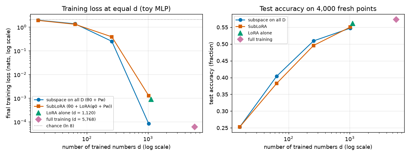
Figure: the toy comparison of output [6].

What this does and does not show:

SubLoRA wins only at the smallest \(d\). From \(d=256\) on, the plain subspace fits better.
In the toy, the LoRA space is only 5.15 times smaller than the full space (1,120 vs 5,768). In GPT-2 small it is 352 times smaller, and the paper uses \(d\le200{,}000\) for 124 million parameters. The toy cannot tell us which method wins at that scale.
So the paper's claim that SubLoRA beats subspace training is an empirical finding at GPT-2 scale (Figure 1, Tables 1–2, one run per setting), not a mathematical consequence of the construction. Nothing in the construction guarantees it; a toy can even reverse it.

Going deeper¶

This section is a hub; the derivations are in the blocks below.

Going deeper: the gradient with respect to w, derived

MY EXPLANATION Write \(\phi(w)=\phi_0+Pw\) and let \(L\) be the training loss. \(L\) depends on \(w\) only through \(\phi\), and \(\partial\phi_i/\partial w_k=P_{ik}\) because \(\phi_0\) and \(P\) are fixed. The chain rule of calculus (Chapter 7) gives, exactly as in Chapter 18,

\[ \frac{\partial L}{\partial w_k}=\sum_{i=1}^{D_{\text{LoRA}}}\frac{\partial L}{\partial\phi_i}\,P_{ik}, \qquad\text{so}\qquad \nabla_wL=P^\top\nabla_\phi L . \]

The vector \(\nabla_\phi L\) is the gradient with respect to all LoRA factors, laid out in the same order as \(\phi\). For one LoRA'd matrix with upstream gradient \(G=\partial L/\partial W\) (shape \(a\times b\)), Chapter 19 derived its two pieces:

\[ \nabla_BL=s\,GA^\top,\qquad \nabla_AL=s\,B^\top G . \]

So the computation is: run the network, backpropagate to each LoRA'd matrix to get \(G\), form these two products, flatten them into one vector in the order of \(\phi\), and multiply by \(P^\top\). Output [5] checks \(\nabla_wL=P^\top\nabla_\phi L\) against PyTorch's automatic differentiation: the largest difference is 0.0.

Units. \(w\), \(\phi\) and \(\theta\) are dimensionless numbers; \(L\) is in nats (the toy) or bits per token (BPD), so every gradient has the units of the loss per unit of \(w\).

Going deeper: proof that the gradient vanishes at w = 0 when the factors start at zero, and grows linearly

MY EXPLANATION Everything here is deterministic: \(\theta_0\), \(\phi_0\), \(P\) are fixed numbers, and we study the loss as a function of \(w\).

Setup. Unflattening is a selection: each entry of \(B_k\) or \(A_k\) is one entry of \(\phi\). So for each LoRA'd matrix \(k\) there are fixed vectors such that, when \(\phi_0=0\),

\[ (B_k)_{ic}=\beta_{ic}^\top w,\qquad (A_k)_{cj}=\gamma_{cj}^\top w, \]

where \(\beta_{ic}^\top\) and \(\gamma_{cj}^\top\) are the rows of \(P\) that feed those entries. Then each entry of the update is

\[ (\Delta W_k)_{ij}=s\sum_{c=1}^{r}(\beta_{ic}^\top w)(\gamma_{cj}^\top w)=w^\top M_{ij}\,w, \qquad M_{ij}=s\sum_{c=1}^{r}\beta_{ic}\gamma_{cj}^\top . \]

So every entry of the update is a quadratic form in \(w\): a sum of products of two coordinates of \(w\), with no constant and no linear term.

Step 1: the update and its derivative vanish at 0. At \(w=0\), \(w^\top M_{ij}w=0\). Its gradient is \((M_{ij}+M_{ij}^\top)w\) (differentiate \(\sum_{p,q}w_p(M_{ij})_{pq}w_q\) with respect to \(w_p\): the \(w_p\) appears in row \(p\) and column \(p\)), which is \(0\) at \(w=0\).

Step 2: the loss gradient vanishes at 0. The loss depends on \(w\) only through the updates, so by the chain rule

\[ \nabla_wL=\sum_k\sum_{i,j}G^{(k)}_{ij}\,(M_{ij}+M_{ij}^\top)\,w , \]

with \(G^{(k)}=\partial L/\partial W_k\) evaluated at the current point. At \(w=0\) every term carries the factor \(w=0\). Hence \(\nabla_wL(0)=0\) for every loss and every data set: \(w=0\) is a stationary point. Gradient descent and Adam (whose step is a function of past gradients, all zero) never move. \(\blacksquare\)

Step 3: linear growth along a ray. Put \(w=\varepsilon u\) with \(\lVert u\rVert=1\). The formula above is \(\varepsilon\,H(\varepsilon u)\,u\) with \(H=\sum_k\sum_{ij}G^{(k)}_{ij}(M_{ij}+M_{ij}^\top)\). As \(\varepsilon\to0\), \(G^{(k)}\) tends to its value at \(\theta_0\) (the network is smooth in its weights, apart from ReLU kinks that a generic \(\theta_0\) does not sit on), so \(\lVert\nabla_wL\rVert/\varepsilon\) tends to the constant \(\lVert H(0)u\rVert\). Output [5] measures this ratio as 0.0098 at \(\varepsilon=10^{-3}\), \(10^{-2}\) and \(10^{-1}\). A small random starting \(w\) would therefore escape, but only slowly at first, and the starting point would no longer be \(\theta_0\) exactly.

Step 4: the fix. With \(\phi_0=(B\text{-parts }0,\ A\text{-parts }A^{(0)})\) the factors are \((B_k)_{ic}=\beta_{ic}^\top w\) and \((A_k)_{cj}=A^{(0)}_{k,cj}+\gamma_{cj}^\top w\). Then

\[ (\Delta W_k)_{ij}=s\sum_c(\beta_{ic}^\top w)\,A^{(0)}_{k,cj}+w^\top M_{ij}w . \]

Now there is a linear term. Its derivative at \(w=0\) is \(s\sum_cA^{(0)}_{k,cj}\beta_{ic}\), and the loss gradient at \(w=0\) is \(\nabla_wL(0)=P^\top g\), where \(g\) holds \(s\,G^{(k)}A^{(0)\top}_k\) in the \(B\)-slots and zeros in the \(A\)-slots (Chapter 19's formulas at \(B=0\)). It is nonzero unless \(g\) happens to be orthogonal to every column of \(P\). Since the \(B\)-parts of \(\phi_0\) are zero, the update at \(w=0\) is still zero, so the model still starts at \(\theta_0\). Output [5]: gradient norm 0.0177.

What is random. \(A^{(0)}\) and \(P\) are drawn once from seeds. For a continuous distribution of \(P\), the event \(P^\top g=0\) for a nonzero \(g\) has probability 0 over the draw of \(P\) (because \(d\ge1\) and a fixed nonzero vector is orthogonal to a random direction with probability 0).

Going deeper: the reachable set is a curved surface of dimension at most d

MY EXPLANATION Define the map \(F(w)=\theta_0+\mathrm{LoRA}(\phi_0+Pw)\) from \(\mathbb R^d\) to \(\mathbb R^{D}\). Its image is the set of networks SubLoRA can reach.

At most \(d\) dimensions. \(F\) is a smooth function of \(d\) numbers, so near any point its image looks like the image of its Jacobian (the \(D\times d\) matrix of first derivatives), which has rank at most \(d\). The description of a point of the image is \(d\) numbers, as for a linear subspace.
Not flat. By the previous block, \(F\) is a polynomial of degree 2 in \(w\). Take the toy case of one matrix, \(r=1\), \(\phi_0=0\): then \(F(w)-\theta_0\) holds \(s\,(\beta^\top w)(\gamma^\top w)\)-type entries, and \(F(2w)-\theta_0=4\,(F(w)-\theta_0)\), not \(2(F(w)-\theta_0)\). A linear map would give 2. With \(\phi_0\neq0\) the map has both a linear and a quadratic part.
Contained in the LoRA set. Every \(F(w)\) is a network whose LoRA'd matrices differ from \(\theta_0\) by rank at most \(r\) (the set \(\mathcal M_r\) of Chapter 19). So SubLoRA searches a \(d\)-dimensional curved surface inside LoRA's \(D_{\text{LoRA}}\)-dimensional curved set, which itself sits inside the full \(D\)-dimensional space.

Why combine at all (an argument, not a theorem). For the same \(d\), a subspace on all parameters and SubLoRA cost the same number of numbers to describe. The difference is where the \(d\) directions point. SubLoRA spends all of them on the matrices LoRA selected (query, value, head) and only on low-rank changes of those, which prior work found to be effective directions (Chapter 19; Hu et al. 2021). A subspace on all parameters spreads them over every weight, bias and layer-norm parameter. Which of the two surfaces passes closer to good networks is an empirical question. PAPER §5, p. 6 The paper's answer for GPT-2 is that SubLoRA is a strict improvement; MY EXPLANATION the toy of step 5 shows the answer can differ for small networks.

The smooth knob. PAPER §1, p. 1 The paper introduces SubLoRA as a way to vary the level of compression smoothly. MY EXPLANATION LoRA's own knob is the rank: \(r=1\to4\) multiplies the count by 4 (87,889 → 351,556). With the subspace on top, \(d\) can take any value up to \(D_{\text{LoRA}}\), and Figure 2 (left) shows the bound as a function of it.

Going deeper: the projector layout at GPT-2 size

[MY EXPLANATION, about SOURCE: authors' code RoundedDoubleKronQR] Chapter 18 showed that the authors build a non-square \(P\) from a Kronecker block of size \(\lfloor\sqrt D\rfloor^2\times\lfloor\sqrt d\rfloor^2\) and a Gaussian remainder block for the leftover rows and columns (erratum E09). If the remainder has fewer rows than columns, some directions of \(w\) satisfy \(Pw=0\) and cannot change the model.

For SubLoRA, \(D=D_{\text{LoRA}}\). Output [3]:

With \(D=351{,}556=592^2+1{,}092\) (real vocabulary), the remainder has 1,092 rows. Every \(d\) of the grid leaves at most 471 remainder columns (at \(d=75{,}000\)), so no direction is lost.
With \(D=351{,}744=593^2+95\) (the code's padded vocabulary), the remainder has only 95 rows. At \(d=50{,}000\) \(=223^2+271\) it has 271 columns, so at least \(271-95=176\) coordinates of \(w\) do nothing (0.35 % of \(w\)). At \(d=75{,}000\) at least 376, at \(d=200{,}000\) at least 96, at \(d=10{,}000\) none (a perfect square).

These dead coordinates still cost bits after quantization, so they can only make the reported bounds slightly worse, never invalid (\(P\) is fixed before training). Whether the authors' runs actually had \(D=351{,}744\) depends on details of their model file that are not in the released excerpt, so this is a plausible reading, not a verified fact.

Paper erratum E57 (same issue as E60): Figure 1's 'complexity' axis is not the second term of Eq. (1)

PAPER Fig. 1 caption, p. 2 The horizontal axis is described as the complexity, "the 2nd term in Equation 1".

MY EXPLANATION The plotted numbers are the two square-root terms of the subsampling bound, Eq. (3): their sum with the risk reproduces Table 1 (12.1224 vs 12.12; output [4]), and the Figure 2 gaps, which reappear as Figure 1 points, match Eq. (3) at \(\alpha=0.25\) to 0.0006 bits per token. At \(d=50{,}000\) the second of these terms is 0.21057 bits per token (ch17_subsampling.py), so Eq. (1)'s term alone would be noticeably smaller than the plotted 1.5278. Impact: labelling only; the bounds are correct.

Paper erratum E58: Figure 2 (left) does not state its fixed hyperparameters

PAPER Fig. 2 caption, p. 5 The caption says the bound is plotted against \(d\) "with LoRA" but not which rank, smoothing level, learning rate or number of quantization levels the runs used.

MY EXPLANATION Output [4] infers the smoothing level: at all eight \(d\) values the plotted complexity matches Eq. (3) only at \(\alpha=0.25\) (the match is within 0.0006, while neighbouring grid values of \(\alpha\) change the interval width \(\Delta\) by about 9 %: from 17.202 bits at \(\alpha=0.25\) to 18.787 at 0.1 and 15.617 at 0.5). Rank and quantization levels cannot be inferred this way. See also erratum E40 for the two extra \(d\) values. Impact: reading only.

Common misconceptions¶

Misconception: SubLoRA trains a small network with \(d\) parameters. — Actually: the network keeps all 123,689,472 parameters and uses all of them in every forward pass. Only \(d\) numbers are free; the rest are fixed by \(\theta_0\), \(\phi_0\) and \(P\), which are regenerated from seeds.
Misconception: In \(P\in\mathbb R^{D\times d}\), \(D\) is the model size. — Actually: \(P\) feeds the LoRA factors, so it has \(D_{\text{LoRA}}\) rows: 351,556 for GPT-2 small at \(r=4\) (351,744 with the code's padded vocabulary), not 123,689,472.
Misconception: Eq. (4) can be implemented exactly as printed. — Actually: with factors equal to \(Pw\) the gradient at \(w=0\) is exactly 0 and training never starts (output [5]; erratum E10). The factors need a fixed random start \(\phi_0\) (\(A\) random, \(B\) zero), as in the authors' code.
Misconception: Combining LoRA with a random subspace must beat a random subspace alone at equal \(d\). — Actually: that is an empirical result for GPT-2 (Figure 1). In the toy of step 5, SubLoRA is better only at \(d=16\) and \(64\); at \(d=256\) the plain subspace reaches 0.2511 nats against 0.3869.
Misconception: Because SubLoRA is "nonlinear", it can reach more networks than LoRA. — Actually: every SubLoRA network is also a LoRA network; SubLoRA reaches a \(d\)-dimensional curved surface inside the LoRA set. What it gains is a shorter description, not more reach.
Misconception: The certified SubLoRA model is a good language model. — Actually: its validation BPD is 10.53 against 4.35 for ordinary training of the same architecture (Table 2), and it produces ungrammatical text (§8). The bound certifies this compressed model, not ordinary GPT-2.

Self-test¶

Q1. Figure 2 (left) plots a compressed size of 35.7461 KB at \(d=100{,}000\). With 1 KB = 8,192 bits, how many bits does each entry of \(w\) cost, and how much smaller is this than storing \(w\) as float32?

Answer

\(35.7461\times8{,}192\approx292{,}832\) bits for \(100{,}000\) entries: 2.928 bits per entry. Float32 needs \(32\times100{,}000=3{,}200{,}000\) bits, so the compressed \(w\) is \(3{,}200{,}000/292{,}832\approx10.9\) times smaller (output [2]). The saving comes from quantization (Chapter 21) and arithmetic coding (Chapter 22), not from the subspace.

Q2. A colleague implements Eq. (4) literally, with all LoRA factors equal to \(Pw\), starts at \(w=0\) and trains with Adam. What happens, and why does starting from a small random \(w\) only partly fix it?

Answer

Every update \(sB_kA_k\) is a quadratic form in \(w\), so its gradient is linear in \(w\) and zero at \(w=0\). The loss gradient is therefore exactly zero, Adam's steps are zero, and the loss stays at its initial value (output [5]: 2.1202 nats after 100 steps). From \(w=\varepsilon u\) the gradient is about \(0.0098\,\varepsilon\) in the toy (output [5]): nonzero but tiny, so training starts very slowly, and the model no longer starts exactly at \(\theta_0\). The authors' fix, a fixed nonzero \(\phi_0\) with \(A\) random and \(B\) zero, gives a gradient of normal size (0.0177) while keeping the start at \(\theta_0\).

Q3. In Figure 1 (left), the best LoRA-only run has BPD risk 11.4091 and complexity 1.6856, and its best top-1 point has risk 0.9078 and complexity 0.0980. Is each bound vacuous? Use \(V=50{,}257\).

Answer

BPD: \(11.4091+1.6856=13.0947<\log_2 50{,}257=15.617\), so it is non-vacuous (it is outside the shaded region). Top-1: \(0.9078+0.0980=1.0058\), which exceeds the random-guess error \(1-1/V\) (just below 1), and even exceeds 1, so it is vacuous; Table 1 reports it as 100. (Output [4].) The LoRA model predicts well on training data but costs too many bits, and the top-1 loss, whose range is only 1, leaves no room for a complexity of 0.098.

Code for this chapter¶

Run it from the project root (about 30–60 s on a laptop CPU):

.venv/Scripts/python explainer/code/ch20_sublora.py

Source: ch20_sublora.py

"""Chapter 20 demo -- SubLoRA: theta = theta0 + LoRA(phi0 + P w)  (paper Sec. 5, Eq. 4, p. 6).

Claims reproduced / checked (every number quoted in Chapter 20 is printed here):
  [1] GPT-2 small bookkeeping: full parameter count D_full (nanoGPT count, pacbound.gpt2_params), LoRA count D_LoRA
      for r = 1, 4 on W_Q, W_V (12 layers) and the head [PAPER App. E], with V = 50,257 [SOURCE: GPT-2 tokenizer]
      and with nanoGPT's padded 50,304 [SOURCE: nanoGPT / authors' code]; the compression ladder
      D_full -> D_LoRA -> d for the App. E grid of d plus the two extra Fig. 2 values (erratum E40).
  [2] What is actually stored: 32 d bits for float32 w vs the compressed sizes plotted in Fig. 2 (left), read
      exactly from the PDF by fig_extract.py (1 KB = 8192 bits, erratum E35), in bits per coordinate of w.
  [3] The authors' non-square projector layout (Ch. 18) applied to D = D_LoRA: remainder-block shapes and the number
      of coordinates of w that cannot affect the model [MY ANALYSIS of SOURCE: authors' code, RoundedDoubleKronQR].
  [4] Figure 1 (left) and Figure 2 (left) read from fig_extract.json: best bound per method, the vacuous line
      (empirical risk + complexity = log2 V), how many plotted runs fall in the vacuous region; Fig. 2's complexity
      (bound - empirical risk) vs d, and the same complexity recomputed from the plotted compressed size with
      Eq. (3) (pacbound.eq3_terms; delta, m [SOURCE: authors' code / nanoGPT]) for each alpha of the grid.
  [5] Zero-gradient caveat (erratum E10) on a toy MLP: with phi0 = 0 the gradient wrt w at w = 0 is exactly 0, and
      it grows linearly in |w| (the update is quadratic in w); with the standard phi0 (A random, B zero) it is not 0;
      chain-rule check grad_w = P^T grad_phi against autograd.
  [6] Toy comparison at equal trainable dimension d in {16, 64, 256, 1024}: (a) linear subspace on all parameters,
      (b) SubLoRA, (c) LoRA alone (all its parameters free), (d) full training; final training loss (nats) and test
      accuracy. Figure: explainer/docs/assets/fig/ch20_param_compare.png
Deterministic (torch.manual_seed / Generator seeds); CPU only; about 30-60 s.
"""
from __future__ import annotations

import json
import math
import sys
import time
from pathlib import Path

HERE = Path(__file__).resolve().parent
sys.path.insert(0, str(HERE))

import matplotlib  # noqa: E402

matplotlib.use("Agg")
import matplotlib.pyplot as plt  # noqa: E402
import torch  # noqa: E402
import torch.nn.functional as F  # noqa: E402

import pacbound as pb  # noqa: E402

T0 = time.time()
torch.set_num_threads(4)
OUT_TXT = HERE / "outputs" / "ch20_sublora.txt"
FIG = HERE.parent / "docs" / "assets" / "fig" / "ch20_param_compare.png"
OUT_TXT.parent.mkdir(exist_ok=True)
FIG.parent.mkdir(parents=True, exist_ok=True)
lines: list[str] = []


def out(s: str = "") -> None:
    print(s)
    lines.append(s)


out("Chapter 20 -- SubLoRA (ch20_sublora.py)")

# ------------------------------------------------------------------------------------------------ [1] bookkeeping
D_FULL = pb.gpt2_params(12, 768)          # nanoGPT count (padded vocab, no position embedding), as in Ch. 5/18/19
assert D_FULL == 123_689_472
KB = 8192                                 # bits per KB (erratum E35)


def lora_count(r: int, V: int, n_layer: int = 12, dm: int = 768) -> int:
    return n_layer * 2 * r * (dm + dm) + r * (dm + V)


D_GRID_FIG2 = [5000, 7500, 10000, 25000, 50000, 75000, 100000, 200000]   # Fig. 2 points; App. E lists 6 (E40)
out(f"[1] GPT-2 small: D_full = {D_FULL:,} parameters (nanoGPT count; ch05_param_count.py)")
for r in (1, 4):
    a, b = lora_count(r, pb.V_GPT2), lora_count(r, 50304)
    out(f"    LoRA r = {r} on W_Q, W_V (12 layers) + head: D_LoRA = {a:,} (V = 50,257) | {b:,} (padded 50,304)"
        f" | D_full / D_LoRA = {D_FULL / a:,.0f}x")
D_L = lora_count(4, pb.V_GPT2)
assert D_L == 351_556 and lora_count(4, 50304) == 351_744
FX = json.loads((HERE / "outputs" / "fig_extract.json").read_text(encoding="utf-8"))
f2 = FX["figure2"]["left"]
kb = [p["value"] for p in f2["compressed_size_kb"]]
risk = [p["value"] for p in f2["empirical_risk"]]
bound = [p["value"] for p in f2["bound"]]
out(f"[2] ladder at r = 4 (D_LoRA = {D_L:,}) and what is stored: Fig. 2 (left) compressed size, 1 KB = 8192 bits; * = d not in App. E grid (E40)")
out("        d    D_LoRA/d   D_full/d   32d bits   plotted KB  plotted bits  bits/coord  float32/plotted")
for d, k in zip(D_GRID_FIG2, kb):
    star = " " if d in pb.D_GRID else "*"
    bits = k * KB
    out(f"    {d:>7,}{star} {D_L / d:7.1f}x {D_FULL / d:8,.0f}x {32 * d:>10,} {k:10.4f} {bits:12,.0f} {bits / d:10.3f} {32 * d / bits:12.1f}x")
out(f"    float32 of all D_full parameters: {32 * D_FULL:,} bits = {32 * D_FULL / KB:,.0f} KB"
    f" = {32 * D_FULL / (kb[4] * KB):,.0f}x the d = 50,000 model's {kb[4]:.4f} KB")

# ------------------------------------------------------------------------------------------------ [3] layout
out("[3] authors' projector layout (Ch. 18) with D = D_LoRA: Kronecker part floor(sqrt D)^2, remainder block")
for Dv in (D_L, lora_count(4, 50304)):
    s = math.isqrt(Dv)
    rows = Dv - s * s
    cells = []
    for d in D_GRID_FIG2:
        t = math.isqrt(d)
        cols = d - t * t
        dead = cols if rows == 0 else max(0, cols - rows)
        cells.append(f"{d / 1000:g}k:{rows}x{cols}" + (f"(>={dead} dead = {dead / d:.2%})" if dead and d == 50000
                                                     else f"(>={dead} dead)" if dead else ""))
    out(f"    D = {Dv:,} = {s}^2 + {rows}: " + ", ".join(cells))

# ------------------------------------------------------------------------------------------------ [4] figures
LOG2V = pb.random_guess_bpd()
f1 = FX["figure1"]
out(f"[4] Figure 1 (left), points read from the PDF (fig_extract.py); vacuous line: risk + complexity = log2 V "
    f"= {LOG2V:.3f}")
poly = f1["left_bpd"]["vacuous_polygon"][0]
edge = [(x, y) for x, y in poly if y < 15.9]
err = max(abs(x + y - LOG2V) for x, y in edge)
out(f"    shaded-region edge vs the line x + y = log2 V: max deviation {err:.4f} BPD over {len(edge)} vertices")
assert err < 0.01
for panel, base, unit in (("left_bpd", LOG2V, "BPD"), ("left_top1", pb.random_guess_topk_error(1), "top-1")):
    for meth, pts in f1[panel]["points"].items():
        bst = min(pts, key=lambda p: p["sum"])
        nvac = sum(p["sum"] >= base for p in pts)
        out(f"    {unit:5s} {meth:8s}: {len(pts):2d} runs, best = {bst['train_risk']:.4f} + {bst['complexity']:.4f}"
            f" = {bst['sum']:.4f}; vacuous runs {nvac}/{len(pts)}")
best_bpd = {m: min(p["sum"] for p in pts) for m, pts in f1["left_bpd"]["points"].items()}
assert abs(best_bpd["SubLoRA"] - 12.12) < 0.005 and abs(best_bpd["LoRA"] - 13.09) < 0.005
assert abs(best_bpd["Subspace"] - 14.59) < 0.005
out(f"    paper Table 1: 12.12 / 13.09 / 14.59 -> diffs {best_bpd['SubLoRA'] - 12.12:+.4f} "
    f"{best_bpd['LoRA'] - 13.09:+.4f} {best_bpd['Subspace'] - 14.59:+.4f}")
fig2_sums = sorted(round(b, 3) for b in bound)
sl_sums = sorted(round(p["sum"], 3) for p in f1["left_bpd"]["points"]["SubLoRA"])
shared = sum(1 for b in fig2_sums if b in sl_sums)
out(f"    the 8 Fig. 2 (left) bounds appear among the 24 SubLoRA points of Fig. 1 (left): {shared}/8")
out("    Figure 2 (left): complexity = bound - empirical risk; Eq. (3) complexity from the plotted size for each alpha")
out(f"    (delta = {pb.DELTA} [SOURCE: authors' code], m = {pb.M_DOCS:,} [SOURCE: nanoGPT], n = {pb.N_SUB:,}; "
    "no hyperparameter bits);")
wid = {a: pb.smoothing_interval(a)[2] for a in (0.1, 0.25, 0.5)}
out(f"    interval width Delta: alpha 0.1 -> {wid[0.1]:.3f}, 0.25 -> {wid[0.25]:.3f}, 0.5 -> {wid[0.5]:.3f} bits "
    f"(ratios to 0.25: {wid[0.1] / wid[0.25]:.3f}, {wid[0.5] / wid[0.25]:.3f})")
out("        d   risk    bound   complexity  | Eq.(3) at the best-matching alpha (diff)")
for d, k, rk, bd in zip(D_GRID_FIG2, kb, risk, bound):
    lip = pb.log_inv_prior_nats_from_bits(k * KB)
    cands = []
    for a in pb.ALPHA_GRID:
        width = pb.smoothing_interval(a)[2]
        t1, t2 = pb.eq3_terms(lip, pb.M_DOCS, pb.N_SUB, width=width)
        cands.append((abs(t1 + t2 - (bd - rk)), a, t1 + t2))
    _, a_b, c_b = min(cands)
    out(f"    {d:>7,} {rk:6.3f} {bd:7.3f} {bd - rk:9.4f}   | alpha = {a_b:<6} {c_b:.4f} ({c_b - (bd - rk):+.4f})")
    if d == 50000:
        assert a_b == 0.25 and abs(c_b - (bd - rk)) < 0.001
out(f"    d = 5,000 -> 50,000: risk {risk[4] - risk[0]:+.3f}, complexity {(bound[4] - risk[4]) - (bound[0] - risk[0]):+.3f}"
    f", bound {bound[4] - bound[0]:+.3f} BPD")

# ------------------------------------------------------------------------------------------------ toy setup
DT = torch.float32
IN, HID, OUT_C, N_TR, N_TE, R = 16, 64, 8, 500, 4000, 4
g = torch.Generator().manual_seed(0)
X = torch.randn(N_TR + N_TE, IN, generator=g, dtype=DT)
T1 = torch.randn(IN, 48, generator=g, dtype=DT) * (2 / math.sqrt(IN))
T2 = torch.randn(48, OUT_C, generator=g, dtype=DT) * (3 / math.sqrt(48))
Y = torch.argmax(torch.tanh(X @ T1) @ T2, 1)                 # labels from a fixed random "teacher"
Xtr, Ytr, Xte, Yte = X[:N_TR], Y[:N_TR], X[N_TR:], Y[N_TR:]
SHAPES = [(HID, IN), (HID, HID), (OUT_C, HID)]               # weight matrices (rows = outputs)


def uniform(gen, a, b, scale):
    return (torch.rand(a, b, generator=gen, dtype=DT) * 2 - 1) * scale


g1 = torch.Generator().manual_seed(1)
W0 = [uniform(g1, a, b, math.sqrt(3.0 / b)) for a, b in SHAPES]          # theta0: frozen random weights
b0 = [torch.zeros(a, dtype=DT) for a, _ in SHAPES]                        # biases (frozen in LoRA/SubLoRA)
THETA0 = torch.cat([t.flatten() for t in W0 + b0])
D_TOY = THETA0.numel()
g2 = torch.Generator().manual_seed(2)
A0 = [uniform(g2, R, b, 1 / math.sqrt(b)) for _, b in SHAPES]             # phi0: A random (loralib-like) ...
B0 = [torch.zeros(a, R, dtype=DT) for a, _ in SHAPES]                     # ... and B zero
FACTORS = [t for pair in zip(B0, A0) for t in pair]                       # flatten order: B1, A1, B2, A2, B3, A3
PHI0 = torch.cat([t.flatten() for t in FACTORS])
D_LT = PHI0.numel()


def unflatten(v, likes):
    parts, i = [], 0
    for t in likes:
        parts.append(v[i:i + t.numel()].view_as(t))
        i += t.numel()
    return parts


def forward(Ws, bs, x):
    h = x
    for k, (W, bb) in enumerate(zip(Ws, bs)):
        h = h @ W.T + bb
        if k < len(Ws) - 1:
            h = torch.relu(h)
    return h


def net_full(theta):                       # theta = theta0 + (change), all D parameters
    p = unflatten(theta, W0 + b0)
    return p[:3], p[3:]


def net_lora(phi):                         # LoRA(phi): unflatten -> W0 + B A per matrix -> biases unchanged
    p = unflatten(phi, FACTORS)
    return [W0[k] + p[2 * k] @ p[2 * k + 1] for k in range(3)], b0


def loss_of(Ws_bs, x=Xtr, y=Ytr):
    return F.cross_entropy(forward(*Ws_bs, x), y)


def qr_projector(rows, cols, seed):
    gg = torch.Generator().manual_seed(seed)
    Q, _ = torch.linalg.qr(torch.randn(rows, cols, generator=gg, dtype=DT))
    return Q                                # dense QR-orthonormal: P^T P = I (Kronecker version: Ch. 18)


# ------------------------------------------------------------------------------------------------ [5] zero gradient
out(f"[5] toy MLP {IN}-{HID}-{HID}-{OUT_C} (ReLU), {N_TR:,} training points labelled by a random teacher; "
    f"D = {D_TOY:,}; LoRA r = {R} on all 3 weight matrices: D_LoRA = {D_LT:,} (D / D_LoRA = {D_TOY / D_LT:.2f})")
P64 = qr_projector(D_LT, 64, 64)


def grad_w(phi0, w):
    w = w.clone().requires_grad_(True)
    L = loss_of(net_lora(phi0 + P64 @ w))
    (gw,) = torch.autograd.grad(L, w)
    return gw, L.item()


w_zero = torch.zeros(64, dtype=DT)
g_std, L_std = grad_w(PHI0, w_zero)
g_nil, L_nil = grad_w(torch.zeros_like(PHI0), w_zero)
out(f"    P: {D_LT} x 64, max |P^T P - I| = {(P64.T @ P64 - torch.eye(64, dtype=DT)).abs().max():.1e};"
    f" at w = 0: loss {L_std:.4f} nats in both cases (the model is theta0)")
out(f"    standard phi0 (A random, B = 0): ||grad_w L|| = {g_std.norm():.4f}")
out(f"    phi0 = 0 (Eq. 4 read literally):  ||grad_w L|| = {g_nil.norm():.1f} (exactly zero: {bool((g_nil == 0).all())})")
assert bool((g_nil == 0).all()) and g_std.norm() > 0.01
gu = torch.Generator().manual_seed(5)
u = torch.randn(64, generator=gu, dtype=DT)
u /= u.norm()
for eps in (1e-3, 1e-2, 1e-1):
    gn, _ = grad_w(torch.zeros_like(PHI0), eps * u)
    out(f"    phi0 = 0, w = {eps:g} * u (unit u): ||grad_w L|| = {gn.norm():.3e}   ratio to eps = {gn.norm() / eps:.4f}")
# chain-rule check: grad_w = P^T grad_phi
phi = (PHI0 + P64 @ (0.1 * u)).clone().requires_grad_(True)
(gphi,) = torch.autograd.grad(loss_of(net_lora(phi)), phi)
gw_auto, _ = grad_w(PHI0, 0.1 * u)
out(f"    chain rule grad_w L = P^T grad_phi L vs autograd: max diff {(P64.T @ gphi - gw_auto).abs().max():.1e}")


def train_w(make, n, lr, steps, w_init=None):
    w = torch.zeros(n, dtype=DT) if w_init is None else w_init.clone()
    w.requires_grad_(True)
    opt = torch.optim.Adam([w], lr=lr)
    for _ in range(steps):
        L = loss_of(make(w))
        opt.zero_grad()
        L.backward()
        opt.step()
    with torch.no_grad():
        Ltr = loss_of(make(w)).item()
        acc = (forward(*make(w), Xte).argmax(1) == Yte).double().mean().item()
    return Ltr, acc, w.detach()


Ls, _, _ = train_w(lambda w: net_lora(PHI0 + P64 @ w), 64, 0.1, 100)
Ln, _, wn = train_w(lambda w: net_lora(torch.zeros_like(PHI0) + P64 @ w), 64, 0.1, 100)
out(f"    100 Adam steps (lr 0.1) from w = 0: standard phi0 {L_std:.4f} -> {Ls:.4f}; "
    f"phi0 = 0 {L_nil:.4f} -> {Ln:.4f} (||w|| = {wn.norm():.1f})")
assert Ln == L_nil and Ls < L_std

# ------------------------------------------------------------------------------------------------ [6] comparison
STEPS, LRS = 150, (0.03, 0.1, 0.3)
D_TOYS = [16, 64, 256, 1024]


def best_of(make, n):
    runs = [train_w(make, n, lr, STEPS)[:2] + (lr,) for lr in LRS]
    return min(runs)                        # smallest final training loss over the learning-rate grid


out(f"[6] equal trainable dimension d; Adam, {STEPS} full-batch steps from w = 0, best of lr in {LRS};")
init_loss = loss_of((W0, b0)).item()
full = best_of(lambda th: net_full(THETA0 + th), D_TOY)
lora = best_of(lambda v: net_lora(PHI0 + v), D_LT)
out("    training cross-entropy in nats (chance ln 8 = %.4f; at theta0 %.4f); test accuracy on %s fresh points "
    "(majority class %.3f)" % (math.log(OUT_C), init_loss, f"{N_TE:,}", torch.bincount(Yte).max().item() / N_TE))
out(f"    full training   (d = D = {D_TOY:,}): loss {full[0]:.4f}  test acc {full[1]:.3f}  (lr {full[2]})")
out(f"    LoRA alone      (d = D_LoRA = {D_LT:,}): loss {lora[0]:.4f}  test acc {lora[1]:.3f}  (lr {lora[2]})")
out(f"    two random projectors per (method, d); mean of the two (each: loss / lr)")
out("        d | subspace on all D: mean loss  acc  (runs)        | SubLoRA: mean loss  acc  (runs)          | lower")
res = {}
for d in D_TOYS:
    subs, sls = [], []
    for sd in (0, 1):
        P_all = qr_projector(D_TOY, d, 1000 * sd + 100 + d)
        P_lo = qr_projector(D_LT, d, 1000 * sd + 200 + d)
        subs.append(best_of(lambda w: net_full(THETA0 + P_all @ w), d))
        sls.append(best_of(lambda w: net_lora(PHI0 + P_lo @ w), d))
    sub = (sum(x[0] for x in subs) / 2, sum(x[1] for x in subs) / 2)
    sl = (sum(x[0] for x in sls) / 2, sum(x[1] for x in sls) / 2)
    res[d] = (sub, sl)
    win = "SubLoRA" if sl[0] < sub[0] else "subspace"
    rs = " ".join(f"{x[0]:.3f}/{x[2]}" for x in subs)
    rl = " ".join(f"{x[0]:.3f}/{x[2]}" for x in sls)
    out(f"    {d:>5} |         {sub[0]:.4f} {sub[1]:.3f} ({rs:<22}) |      {sl[0]:.4f} {sl[1]:.3f} ({rl:<22}) | {win}")

fig, ax = plt.subplots(1, 2, figsize=(10.5, 4.0))
ax[0].plot(D_TOYS, [res[d][0][0] for d in D_TOYS], "o-", color="#0072B2", label="subspace on all D (θ0 + Pw)")
ax[0].plot(D_TOYS, [res[d][1][0] for d in D_TOYS], "s-", color="#D55E00", label="SubLoRA (θ0 + LoRA(φ0 + Pw))")
ax[0].plot([D_LT], [lora[0]], "^", color="#009E73", ms=9, label=f"LoRA alone (d = {D_LT:,})")
ax[0].plot([D_TOY], [full[0]], "D", color="#CC79A7", ms=8, label=f"full training (d = {D_TOY:,})")
ax[0].axhline(math.log(OUT_C), color="grey", ls=":", lw=1, label="chance (ln 8)")
ax[0].set_xscale("log")
ax[0].set_yscale("log")
ax[0].set_xlabel("number of trained numbers d (log scale)")
ax[0].set_ylabel("final training loss (nats, log scale)")
ax[0].set_title("Training loss at equal d (toy MLP)")
ax[0].legend(fontsize=8)
ax[1].plot(D_TOYS, [res[d][0][1] for d in D_TOYS], "o-", color="#0072B2", label="subspace on all D")
ax[1].plot(D_TOYS, [res[d][1][1] for d in D_TOYS], "s-", color="#D55E00", label="SubLoRA")
ax[1].plot([D_LT], [lora[1]], "^", color="#009E73", ms=9, label="LoRA alone")
ax[1].plot([D_TOY], [full[1]], "D", color="#CC79A7", ms=8, label="full training")
ax[1].set_xscale("log")
ax[1].set_xlabel("number of trained numbers d (log scale)")
ax[1].set_ylabel("test accuracy (fraction)")
ax[1].set_title("Test accuracy on 4,000 fresh points")
ax[1].legend(fontsize=8)
for a in ax:
    a.grid(alpha=0.3)
fig.tight_layout()
fig.savefig(FIG, dpi=130)
print(f"Figure: {FIG.name}")
print(f"Runtime {time.time() - T0:.0f} s (CPU)")
OUT_TXT.write_text("\n".join(lines) + "\n", encoding="utf-8")

Output:

Chapter 20 -- SubLoRA (ch20_sublora.py)
[1] GPT-2 small: D_full = 123,689,472 parameters (nanoGPT count; ch05_param_count.py)
    LoRA r = 1 on W_Q, W_V (12 layers) + head: D_LoRA = 87,889 (V = 50,257) | 87,936 (padded 50,304) | D_full / D_LoRA = 1,407x
    LoRA r = 4 on W_Q, W_V (12 layers) + head: D_LoRA = 351,556 (V = 50,257) | 351,744 (padded 50,304) | D_full / D_LoRA = 352x
[2] ladder at r = 4 (D_LoRA = 351,556) and what is stored: Fig. 2 (left) compressed size, 1 KB = 8192 bits; * = d not in App. E grid (E40)
        d    D_LoRA/d   D_full/d   32d bits   plotted KB  plotted bits  bits/coord  float32/plotted
      5,000     70.3x   24,738x    160,000     2.1124       17,305      3.461          9.2x
      7,500*    46.9x   16,492x    240,000     2.5564       20,942      2.792         11.5x
     10,000     35.2x   12,369x    320,000     3.8782       31,770      3.177         10.1x
     25,000     14.1x    4,948x    800,000     9.8081       80,348      3.214         10.0x
     50,000      7.0x    2,474x  1,600,000    16.5325      135,434      2.709         11.8x
     75,000*     4.7x    1,649x  2,400,000    27.9915      229,307      3.057         10.5x
    100,000      3.5x    1,237x  3,200,000    35.7461      292,832      2.928         10.9x
    200,000      1.8x      618x  6,400,000    57.3441      469,763      2.349         13.6x
    float32 of all D_full parameters: 3,958,063,104 bits = 483,162 KB = 29,225x the d = 50,000 model's 16.5325 KB
[3] authors' projector layout (Ch. 18) with D = D_LoRA: Kronecker part floor(sqrt D)^2, remainder block
    D = 351,556 = 592^2 + 1092: 5k:1092x100, 7.5k:1092x104, 10k:1092x0, 25k:1092x36, 50k:1092x271, 75k:1092x471, 100k:1092x144, 200k:1092x191
    D = 351,744 = 593^2 + 95: 5k:95x100(>=5 dead), 7.5k:95x104(>=9 dead), 10k:95x0, 25k:95x36, 50k:95x271(>=176 dead = 0.35%), 75k:95x471(>=376 dead), 100k:95x144(>=49 dead), 200k:95x191(>=96 dead)
[4] Figure 1 (left), points read from the PDF (fig_extract.py); vacuous line: risk + complexity = log2 V = 15.617
    shaded-region edge vs the line x + y = log2 V: max deviation 0.0000 BPD over 100 vertices
    BPD   SubLoRA : 24 runs, best = 10.5945 + 1.5278 = 12.1224; vacuous runs 0/24
    BPD   LoRA    :  4 runs, best = 11.4091 + 1.6856 = 13.0947; vacuous runs 2/4
    BPD   Subspace: 12 runs, best = 13.8138 + 0.7758 = 14.5896; vacuous runs 1/12
    top-1 SubLoRA : 24 runs, best = 0.9148 + 0.0494 = 0.9641; vacuous runs 8/24
    top-1 LoRA    :  4 runs, best = 0.9078 + 0.0980 = 1.0058; vacuous runs 4/4
    top-1 Subspace: 12 runs, best = 0.9037 + 0.0616 = 0.9652; vacuous runs 4/12
    paper Table 1: 12.12 / 13.09 / 14.59 -> diffs +0.0024 +0.0047 -0.0004
    the 8 Fig. 2 (left) bounds appear among the 24 SubLoRA points of Fig. 1 (left): 8/8
    Figure 2 (left): complexity = bound - empirical risk; Eq. (3) complexity from the plotted size for each alpha
    (delta = 0.05 [SOURCE: authors' code], m = 8,009,762 [SOURCE: nanoGPT], n = 10,000; no hyperparameter bits);
    interval width Delta: alpha 0.1 -> 18.787, 0.25 -> 17.202, 0.5 -> 15.617 bits (ratios to 0.25: 1.092, 0.908)
        d   risk    bound   complexity  | Eq.(3) at the best-matching alpha (diff)
      5,000 11.833  12.516    0.6824   | alpha = 0.25   0.6819 (-0.0006)
      7,500 11.659  12.388    0.7294   | alpha = 0.25   0.7289 (-0.0005)
     10,000 11.365  12.215    0.8492   | alpha = 0.25   0.8488 (-0.0004)
     25,000 10.934  12.160    1.2254   | alpha = 0.25   1.2251 (-0.0002)
     50,000 10.595  12.122    1.5278   | alpha = 0.25   1.5276 (-0.0002)
     75,000 10.967  12.891    1.9244   | alpha = 0.25   1.9242 (-0.0001)
    100,000 10.363  12.510    2.1472   | alpha = 0.25   2.1471 (-0.0001)
    200,000 10.364  13.027    2.6633   | alpha = 0.25   2.6632 (-0.0001)
    d = 5,000 -> 50,000: risk -1.239, complexity +0.845, bound -0.393 BPD
[5] toy MLP 16-64-64-8 (ReLU), 500 training points labelled by a random teacher; D = 5,768; LoRA r = 4 on all 3 weight matrices: D_LoRA = 1,120 (D / D_LoRA = 5.15)
    P: 1120 x 64, max |P^T P - I| = 4.2e-07; at w = 0: loss 2.1202 nats in both cases (the model is theta0)
    standard phi0 (A random, B = 0): ||grad_w L|| = 0.0177
    phi0 = 0 (Eq. 4 read literally):  ||grad_w L|| = 0.0 (exactly zero: True)
    phi0 = 0, w = 0.001 * u (unit u): ||grad_w L|| = 9.813e-06   ratio to eps = 0.0098
    phi0 = 0, w = 0.01 * u (unit u): ||grad_w L|| = 9.813e-05   ratio to eps = 0.0098
    phi0 = 0, w = 0.1 * u (unit u): ||grad_w L|| = 9.815e-04   ratio to eps = 0.0098
    chain rule grad_w L = P^T grad_phi L vs autograd: max diff 0.0e+00
    100 Adam steps (lr 0.1) from w = 0: standard phi0 2.1202 -> 1.4389; phi0 = 0 2.1202 -> 2.1202 (||w|| = 0.0)
[6] equal trainable dimension d; Adam, 150 full-batch steps from w = 0, best of lr in (0.03, 0.1, 0.3);
    training cross-entropy in nats (chance ln 8 = 2.0794; at theta0 2.1202); test accuracy on 4,000 fresh points (majority class 0.221)
    full training   (d = D = 5,768): loss 0.0001  test acc 0.573  (lr 0.1)
    LoRA alone      (d = D_LoRA = 1,120): loss 0.0009  test acc 0.562  (lr 0.1)
    two random projectors per (method, d); mean of the two (each: loss / lr)
        d | subspace on all D: mean loss  acc  (runs)        | SubLoRA: mean loss  acc  (runs)          | lower
       16 |         1.9551 0.253 (1.943/0.1 1.967/0.3   ) |      1.9111 0.253 (1.910/0.1 1.912/0.3   ) | SubLoRA
       64 |         1.3738 0.404 (1.364/0.3 1.384/0.3   ) |      1.3127 0.383 (1.318/0.3 1.307/0.1   ) | SubLoRA
      256 |         0.2511 0.509 (0.249/0.3 0.253/0.1   ) |      0.3869 0.496 (0.382/0.1 0.391/0.1   ) | subspace
     1024 |         0.0001 0.547 (0.000/0.3 0.000/0.3   ) |      0.0013 0.551 (0.001/0.1 0.002/0.03  ) | subspace