04. Language models¶
Where this fits
Prerequisites: Chapter 1 (probability, distribution, conditional probability, independence, expectation), Chapter 3 (ln, \(\log_2\), bits, nats, surprisal). We also use the words model, parameter, training and dataset from Chapter 2. Used later by: Chapter 5 (the network that computes the probabilities), Chapter 6 (scoring a language model), Chapter 15 (why documents, not tokens, are the independent units), Chapter 16 (prediction smoothing), Chapter 24 (long documents), Chapter 26 and Chapter 28. Purpose: say exactly what kind of object the paper's bounds are about — a machine that gives a probability to every possible next piece of text.
The problem this chapter solves¶
Everything in this section is MY EXPLANATION unless tagged.
PAPER Abstract and §1, p. 1 The paper proves bounds for large language models (LLMs) that were trained on "next token prediction". The first difficulty it lists is that LLMs are trained on autoregressive token prediction, so their token predictions are not independent.
That sentence uses four words we have not met: language model, token, next token prediction and autoregressive. Every formula in the paper is written in their terms.
A language model is a model (Chapter 2) that gives a probability to every piece of text. A large language model (LLM) is a language model with a very large number of parameters, trained on a very large amount of text.
PAPER App. E, p. 16 The paper's main model, GPT-2 small, has 124 million parameters.
PAPER §4.3, p. 5 The paper writes the probability that its model gives to a whole document \(X\) of \(L\) tokens as a product, \(p_h(X) = \prod_{i=1}^{L} p_h(x_i \mid x_{<i})\).
MY EXPLANATION Here a document is one self-contained piece of text, such as one web page, and a token is roughly a word or a piece of a word. The next sections make both precise.
To read that one line we must answer five questions:
- What does a language model read and predict? (Tokens, made by a tokenizer.)
- Why is the probability of a whole document a product? (The chain rule of probability.)
- Where do the probabilities come from, and how small can they get? (Logits and softmax.)
- How much of the past can the model see? (The context window.)
- How does a model write text, and what does "temperature 0.8" in the paper's appendix mean? (Sampling.)
This chapter answers all five. It then builds a complete, tiny language model by counting letters, so that every idea has real numbers attached.
Intuition (and where the analogy breaks)¶
Everything in this section is MY EXPLANATION unless tagged.
Think of the autocomplete on a phone keyboard. You type "see you". It suggests "tomorrow", "soon", "later". It has guessed what usually comes next, given what you typed so far.
Now imagine a storyteller who writes a story one piece at a time. Before each piece, she looks at the story so far. Then she rolls a loaded die. The die has one face for every possible next piece. Its weights depend on the story so far: after "once upon a", the face "time" is very heavy.
She writes down whatever the die shows, and repeats. That is how a language model writes text.
The same die also scores text. Take any finished story. At each step, look up how heavy the die made the piece that was actually written. Multiply those weights together. The result is the probability that the storyteller would have produced exactly this story. A good language model gives high probability to real text.
Where it breaks.
- The memory is short. The storyteller sees the whole story. A real model sees only the most recent pieces, up to a fixed limit called the context window (defined below).
- The pieces are not words. They are tokens: whole words, parts of words, single letters or punctuation marks.
- Nobody keeps a table of dice. There are far too many possible stories to store one die for each. The weights are computed fresh for every situation by a neural network — a large adjustable formula with many parameters, which Chapter 5 describes — using the same parameters every time.
- Autocomplete shows three suggestions. A language model gives a probability to every token in its vocabulary — tens of thousands of them for GPT-2.
Precise definition¶
Everything in this section is MY EXPLANATION unless tagged.
Text, characters and tokens¶
Text is a sequence of characters. A character is one written symbol: a letter, a digit, a punctuation mark, a space, or an invisible symbol such as "new line".
Computers store characters as bytes (a byte is 8 bits, Chapter 3).
SOURCE: UTF-8 standard, RFC 3629 In the common UTF-8 encoding, each English letter takes one byte. Accented letters, Chinese characters or emoji take two to four bytes.
MY EXPLANATION A token is the unit that a language model reads and predicts. It is a short piece of text. Depending on the text, a token can be a single byte, part of a word, a whole word (usually including the space in front of it), or a run of punctuation.
The vocabulary is the fixed, finite list of all tokens a model can use. Its size is written \(V\).
A token id is the position of a token in the vocabulary: a whole number from 0 to \(V-1\). A language model never sees letters. It sees only token ids.
A tokenizer is the fixed program that cuts text into tokens and replaces each token by its id. It also does the reverse: it turns a list of ids back into text. The tokenizer is chosen before the model is trained and never changes.
SOURCE: GPT-2 tokenizer (OpenAI's released files, Radford et al. 2019; tiktoken's "gpt2" encoding) GPT-2's vocabulary has \(V = 50{,}257\) tokens: 256 tokens for the 256 possible byte values, 50,000 tokens built by merging (next subsection), and 1 special token.
Paper erratum E36: V is never printed
PAPER §4.3, p. 5; §6.2, p. 7 The paper writes "a vocabulary of size V", \(\log_2 V\) and \(1 - k/V\), but never gives the value of \(V\).
MY EXPLANATION Every number in this explainer that uses \(V = 50{,}257\) therefore takes it from GPT-2's tokenizer, not from the paper. Chapter 3 shows that the paper's rounded 15.62 agrees with this value.
MY EXPLANATION The special token is the end-of-text token, written <|endoftext|>. It marks where one document ends and the
next begins. Chapter 15 explains why the paper treats whole documents as its basic unit.
[SOURCE: nanoGPT prepare.py] The paper's training data is OpenWebText, a public collection of web pages. nanoGPT,
the training code the paper builds on, turns each OpenWebText document into token ids, appends the end-of-text token
(id 50,256) after it, and joins everything into one long stream. The training split has 8,009,762 documents and
9,035,582,198 tokens.
[SOURCE: authors' code, sublora_sublora_pipeline.py] The authors' code finds the document boundaries in that
stream by searching for id 50,256.
Paper erratum E42: the end-of-text token is garbled in Table 7
PAPER Table 7, p. 19 In the last sample of text generated by the SubLoRA model, the string "¡—endoftext—¿" appears in the middle of the text.
MY EXPLANATION This is GPT-2's end-of-text token <|endoftext|>. In some LaTeX font
encodings, the characters <, | and > typed in ordinary text print as ¡, — and ¿. No number is affected. But a
reader may not recognise that the model emitted an end-of-text token there: it "finished" one document and
started a new one in the middle of the sample.
Byte-pair encoding: where GPT-2's tokens come from¶
How do you choose 50,000 useful tokens? GPT-2 uses byte-pair encoding (BPE). The recipe is short:
- Start with the 256 single bytes as tokens. Write a large training text as a sequence of bytes.
- Count every pair of neighbouring tokens in the text.
- Take the most frequent pair, for example "t" followed by "h". Make it a new token "th". Add it to the vocabulary. Replace every "t h" in the text by "th".
- Repeat steps 2–3. Each repetition (a merge) adds one token.
SOURCE: GPT-2 tokenizer files GPT-2's tokenizer was built with 50,000 merges. That gives 256 + 50,000 = 50,256 ordinary tokens, plus the end-of-text token: 50,257.
MY EXPLANATION Frequent words end up as single tokens. Rare words are spelled with several pieces. Any text at all can be written, because in the worst case every byte is its own token. The worked example below runs 10 merges on a short paragraph.
Going deeper: byte-pair encoding precisely, and GPT-2's version
MY EXPLANATION Learning the merges. Input: a training text, a base alphabet \(B\) (for GPT-2, the 256 byte values), and a number of merges \(M\).
- Split the text into chunks that merges may not cross, and write each chunk as a sequence of base symbols.
- For \(r = 1, 2, \dots, M\): count every adjacent pair \((a, b)\) inside the chunks. Pick the most frequent pair (some fixed tie rule is needed). Create the new symbol \(ab\), add it to the vocabulary, and record the rule "\(a + b \to ab\)" with rank \(r\). Scan each chunk from left to right and replace every occurrence of \(a\) followed by \(b\) by \(ab\) (occurrences do not overlap).
The vocabulary ends with \(|B| + M\) symbols, plus any special tokens. For GPT-2: \(256 + 50{,}000 + 1 = 50{,}257\).
Encoding new text. Write the new text as base symbols. Among the adjacent pairs that have a rule, find the one with the lowest rank (the one learned first) and merge it. Repeat until no adjacent pair has a rule.
[SOURCE: OpenAI GPT-2 code, encoder.py] GPT-2's released encoder works this way.
MY EXPLANATION Decoding. Each token stands for a fixed string of bytes. Concatenate the bytes of the tokens and read them as UTF-8 text. Since merging only glues neighbours together, decoding an encoded text returns the original text exactly.
Why bytes. Every text in every language is a sequence of bytes. So a byte-level tokenizer never meets an "unknown" character. A rare character just costs several tokens, one per byte at worst.
SOURCE: Radford et al. 2019, §2.2 GPT-2 does not let BPE merge across character categories (letters, digits, punctuation), with one exception: a space may join the word that follows it. That is why GPT-2's tokens look like "␣the" (space first).
MY EXPLANATION Our toy example below has no such rule, so it learns tokens such as "e␣" and "␣the␣" that cross word boundaries.
MY ANALYSIS The tokenizer and the bound. The paper never discusses the tokenizer's role in the bound. It reuses GPT-2's tokenizer unchanged. That tokenizer was built by OpenAI for GPT-2, before and separately from this paper's experiments, and training never changes it. So it can be treated as part of the fixed setup that the paper's prior takes as given, like the architecture. (The prior is the probability the bound assigns to each model before seeing any data; Chapters 11 and 13 make it precise.) A tokenizer tuned on the very documents used in the bound would be a hidden choice made after seeing the data.
A document as a sequence of tokens¶
From now on a document is a sequence of token ids,
Here \(x_i\) is the \(i\)-th token and \(L\) is the number of tokens. We write \(x_{<i}\) for all tokens before position \(i\), that is \((x_1, \dots, x_{i-1})\). For \(i = 1\) this is the empty sequence: nothing has been seen yet.
PAPER §4.3, p. 5; App. E, p. 16 The paper uses the same \(x_i\) and \(x_{<i}\) in §4.3. Appendix E writes the same prefix as \(x_{:i-1}\).
The chain rule of probability¶
MY EXPLANATION Here is the key fact. For any probability distribution over sequences,
In words: the probability of the whole sequence is the probability of the first token, times the probability of the second token given the first, times the probability of the third given the first two, and so on. The symbol \(\prod_{i=1}^{L}\) means "multiply the following factor over \(i = 1, 2, \dots, L\)". The bar "\(\mid\)" is the conditional probability of Chapter 1: "given that the earlier tokens were these".
This is the chain rule of probability. It needs no assumption at all about how the tokens relate to each other.
Taking \(\log_2\) turns the product into a sum (product rule of logarithms, Chapter 3):
The left side is the surprisal of the whole document, in bits. The right side adds up the surprisals of its tokens, each measured in its own context. Chapter 6 divides this sum by \(L\) to get the paper's main loss (bits per token).
Going deeper: proof of the chain rule
MY EXPLANATION Setup. Let \((X_1, \dots, X_L)\) be a random sequence of tokens with any joint distribution (Chapter 1). Fix particular tokens \(x_1, \dots, x_L\). For \(i = 1, \dots, L\) let \(A_i\) be the event "the first \(i\) tokens are \(x_1, \dots, x_i\)", and let \(A_0 = \Omega\) (the whole sample space: no condition). Each event is contained in the one before: \(A_0 \supseteq A_1 \supseteq \cdots \supseteq A_L\). In this notation, \(p(x_1, \dots, x_i) = \Pr[A_i]\) and \(p(x_i \mid x_{<i}) = \Pr[A_i \mid A_{i-1}]\).
Claim. If \(\Pr[A_{L-1}] > 0\), then \(\Pr[A_L] = \prod_{i=1}^{L} \Pr[A_i \mid A_{i-1}]\).
Proof by induction on \(L\). For \(L = 1\): \(\Pr[A_1 \mid A_0] = \Pr[A_1 \cap \Omega]/\Pr[\Omega] = \Pr[A_1]/1 = \Pr[A_1]\).
Now let \(L \ge 2\) and assume the claim for \(L - 1\). Its condition holds, because \(A_{L-1} \subseteq A_{L-2}\) gives \(\Pr[A_{L-2}] \ge \Pr[A_{L-1}] > 0\). Since \(A_L \subseteq A_{L-1}\), we have \(A_L \cap A_{L-1} = A_L\). The definition of conditional probability then reads \(\Pr[A_L \mid A_{L-1}] = \Pr[A_L]/\Pr[A_{L-1}]\). Multiply both sides by \(\Pr[A_{L-1}]\) and use the induction hypothesis:
Edge case: a prefix of probability 0. Let \(j\) be the first index with \(\Pr[A_j] = 0\). The factor \(\Pr[A_j \mid A_{j-1}]\) is defined (because \(\Pr[A_{j-1}] > 0\)) and equals 0. Later factors condition on an event of probability 0, which Chapter 1's definition leaves undefined. A language model, however, supplies a next-token distribution for every prefix. Whatever numbers in \([0, 1]\) fill those later factors, the product is 0, which is the correct value of \(\Pr[A_L]\). So the formula holds in every case when the factors are the model's own conditionals.
What the proof did not use. Nothing about independence. The tokens may depend on each other in any way. The proof also works for any order of revealing the tokens; for example, right to left gives \(p(x_1, \dots, x_L) = \prod_i p(x_i \mid x_{i+1}, \dots, x_L)\). Language models use left to right because that is the order in which text is written and generated.
The log form. If \(\Pr[A_L] > 0\), every factor is positive and the product rule for logarithms gives \(-\log_2 \Pr[A_L] = \sum_i \bigl(-\log_2 \Pr[A_i \mid A_{i-1}]\bigr)\). Each term is a surprisal in bits, so the sum is in bits.
Going deeper: next-token distributions always define a valid distribution, and why the end-of-text token is needed
MY EXPLANATION (a) Fixed length. Suppose that for every prefix \(s\) (a sequence of tokens, possibly empty) we are given a distribution \(q(\cdot \mid s)\) over the vocabulary: \(q(v \mid s) \ge 0\) and \(\sum_v q(v \mid s) = 1\). Define, for sequences of length \(L\),
Claim: \(p_L \ge 0\) and \(\sum p_L(x_1, \dots, x_L) = 1\), where the sum runs over all \(V^L\) sequences.
Proof by induction on \(L\). For \(L = 1\) the sum is \(\sum_{x_1} q(x_1 \mid \text{empty}) = 1\). For \(L \ge 2\), sum over the last token first. Only the last factor depends on \(x_L\):
by the induction hypothesis. \(\blacksquare\)
The same "sum out the last token" step shows that the probability of a prefix \((x_1, \dots, x_i)\) under \(p_L\) is \(\prod_{j \le i} q(x_j \mid x_{<j})\). Dividing two consecutive prefixes, the conditional probabilities of \(p_L\) are exactly the \(q\)'s (wherever the prefix has positive probability). So a family of next-token distributions and a distribution over sequences are the same thing, seen two ways.
(b) Documents of different lengths. Real documents have different lengths. If we added \(p_L\) over all lengths \(L = 1, 2, 3, \dots\), we would get \(1 + 1 + 1 + \cdots\), which is not a probability. The end-of-text token fixes this. Start the model from an end-of-text context; let it produce tokens; stop when it produces end-of-text. A document \((x_1, \dots, x_L)\) of ordinary tokens then has probability
Different documents are different outcomes of one process ("the first stop happens right after exactly these tokens"). These outcomes are disjoint, so their probabilities add up to \(\Pr[\text{the process ever stops}] \le 1\).
The total is exactly 1 if, for example, every prefix gives end-of-text a probability of at least some fixed \(\varepsilon > 0\). Then, by the chain rule, the probability of producing \(n\) tokens without stopping is a product of \(n\) factors, each at most \(1 - \varepsilon\), so it is at most \((1-\varepsilon)^n\), which tends to 0.
[SOURCE: authors' code, sublora_utils.py, sample_single_document] (c) What the paper's code scores.
For the bound, the authors' code takes a document's tokens together with the end-of-text token that precedes it.
It scores every token of the document given its prefix, starting from that end-of-text token. The closing
end-of-text token is not scored.
MY EXPLANATION For the bound this is fine. The bound needs one loss value per document (Chapter 6, Chapter 15), not a normalised distribution over all documents.
MY EXPLANATION Why the tokens of a document are not independent. If tokens were independent, knowing the earlier tokens would not change the probability of the next one: \(p(x_i \mid x_{<i})\) would equal \(p(x_i)\). In real text this is false. In the worked example below, the letter "h" makes up 7.3 % of all symbols, but 54.8 % of the symbols that follow a "t". The conditionals in the chain rule are where all that dependence lives.
PAPER §1, p. 1 This is the paper's challenge (i).
MY EXPLANATION The paper needs independent pieces because Hoeffding's inequality (Chapter 9) is proved for independent random variables. So it does not treat tokens as its examples. It treats whole documents, drawn independently, as the examples; Chapter 15 explains this choice.
Autoregressive language models and next-token prediction¶
An autoregressive model is a model that predicts each element of a sequence from the elements before it. For text: an autoregressive language model is a rule that, for every possible prefix \(x_{<i}\), outputs a probability distribution over the \(V\) tokens of the vocabulary. We write it
where \(\theta\) stands for all the parameters of the model (Chapter 2). "Autoregressive" means "predicted from its own past": each token is predicted from the earlier tokens of the same sequence. When such a model writes text, it feeds its own outputs back in as the new prefix.
Combined with the chain rule, a model of next-token probabilities is automatically a model of whole documents:
PAPER §4.3, p. 5 The paper defines the probability of a document under its model in exactly this way: \(p_h(X) := \prod_{i}^{L} p_h(x_i \mid x_{<i})\). The model \(p_h\) is a slightly modified version of \(p_\theta\) that Chapter 16 introduces.
PAPER App. E, p. 16 Appendix E states the same factorization, \(p(x_{:k}) = \prod_{i=1}^{k} p(x_i \mid x_{:i-1})\).
MY EXPLANATION Next-token prediction is the task these models are trained on. Show the model real text. At every position, it gives a distribution for the next token. It is scored by how much probability it gave to the token that actually came next: a lower surprisal is better. Training adjusts \(\theta\) to lower the total surprisal of the training text.
One document of \(L\) tokens therefore provides \(L\) predictions to learn from. Chapter 6 names this score (negative log-likelihood). Chapter 7 explains how the parameters are adjusted.
PAPER App. E, p. 16 The paper's models are trained this way from scratch on the training split of OpenWebText.
Logits and softmax¶
MY EXPLANATION How does a model output a distribution over its whole vocabulary at once? In two steps.
First, the network (Chapter 5) computes one real number for every token \(v\) in the vocabulary. These numbers are called logits and written \(z_v\). A logit can be any real number, positive or negative. A larger logit means the model favours that token more.
Second, the logits are turned into probabilities by the softmax function:
Here \(e^{z_v}\) is the exponential function of Chapter 3, and \(u\) runs over all \(V\) tokens of the vocabulary. Raising \(e\) to the power \(z_v\) makes every score positive. Dividing by the total makes the scores add up to 1.
Five properties matter for the paper (proofs in the next blocks):
- Every output is positive and the outputs add up to 1, so softmax always gives a valid distribution.
- A larger logit always gives a larger probability. The order of the tokens is kept.
- Adding the same number to every logit changes nothing. Only differences between logits matter.
- In exact arithmetic, no probability is ever exactly 0. But there is no lower limit either. A token whose logit is 20 below the largest one has a surprisal between 28.85 and 44.47 bits (with GPT-2's \(V = 50{,}257\), a value taken from the GPT-2 tokenizer). As the gap grows, the surprisal grows without any ceiling. This is the "unbounded loss" that Chapter 6 and Chapter 16 deal with.
- In a computer's arithmetic, a tiny probability can round to exactly 0.
Going deeper: properties of softmax, with proofs
MY EXPLANATION Let \(z = (z_u)\) be the logits, one real number per token \(u\) of a vocabulary of size \(V\). Let \(S = \sum_u e^{z_u}\) and \(p_v = e^{z_v}/S\).
(i) A valid distribution. \(e^{x} > 0\) for every real \(x\) (Chapter 3), so \(S > 0\) and every \(p_v > 0\). And \(\sum_v p_v = \frac{1}{S}\sum_v e^{z_v} = S/S = 1\).
(ii) Shift invariance. For any real \(c\), the addition law of the exponential gives \(e^{z_v + c} = e^c e^{z_v}\). So \(\mathrm{softmax}(z + c)_v = \dfrac{e^c e^{z_v}}{\sum_u e^c e^{z_u}} = \dfrac{e^c e^{z_v}}{e^c S} = p_v\).
(iii) Ratios and order. \(p_u / p_v = e^{z_u}/e^{z_v} = e^{z_u - z_v}\): only differences of logits matter. Because \(e^x\) is strictly increasing, \(z_u > z_v\) exactly when \(p_u > p_v\). In particular, the token with the largest logit is the token with the largest probability.
(iv) Every strictly positive distribution is a softmax. Let \(q_v > 0\) with \(\sum_v q_v = 1\). Put \(z_v = \ln q_v\). Then \(e^{z_v} = q_v\), \(S = 1\), and \(\mathrm{softmax}(z) = q\). The logits are unique up to a shift: if \(\mathrm{softmax}(z) = \mathrm{softmax}(z')\), then by (iii) \(z_u - z_v = z'_u - z'_v\) for all \(u, v\), so \(z - z'\) is the same number for every token. A probability of exactly 0 would need \(z_v = -\infty\), which is not a real number. Our counting model below uses \(-\infty\) for pairs it never saw; a network that computes finite logits cannot do this.
(v) Log-softmax and its bounds. Taking ln of \(p_v = e^{z_v}/S\) gives
LSE stands for "log-sum-exp". Let \(z_{\max}\) be the largest logit. The sum \(S\) contains the term \(e^{z_{\max}}\) and all its terms are positive, so \(S \ge e^{z_{\max}}\). Each of its \(V\) terms is at most \(e^{z_{\max}}\), so \(S \le V e^{z_{\max}}\). Since ln is increasing,
Let \(g_v = z_{\max} - z_v \ge 0\) be the logit gap of token \(v\). Its surprisal in nats is \(-\ln p_v = \mathrm{LSE}(z) - z_v\). The bounds on LSE give \(g_v \le -\ln p_v \le g_v + \ln V\). Dividing by \(\ln 2\) converts nats to bits:
With \(g_v = 20\) and \(V = 50{,}257\) (GPT-2 tokenizer): between \(20/\ln 2 = 28.85\) and \(28.85 + 15.617 = 44.47\) bits. The surprisal is bounded exactly when the logit gap is bounded, and nothing in an ordinary network bounds the gap. So the per-token loss of a language model has no ceiling. Chapter 16 shows how the paper creates one.
Going deeper: softmax inside a computer
MY EXPLANATION Computers store real numbers in floating-point formats with a finite range. The two common ones are float64 ("double precision") and float32 ("single precision").
Underflow. For very negative \(x\), the true value of \(e^x\) is smaller than the smallest positive number the format can hold, so the computer rounds it to exactly 0. The script finds the thresholds: \(e^x\) becomes 0 for \(x\) below \(-745.13\) in float64 and below \(-103.97\) in float32. So in float64, \(\mathrm{softmax}([0, -800])\) comes out as \([1, 0.0]\), and in float32, \(\mathrm{softmax}([0, -110])\) has a second entry of exactly 0.0.
Overflow. For large \(x\), \(e^x\) exceeds the largest number the format can hold and becomes "inf" (infinity). Then inf/inf gives "nan" (not a number). The script adds 1,000 to the logits of a real distribution and computes softmax naively: 12 entries come out as nan.
The fix uses shift invariance. Subtract \(z_{\max}\) from every logit before exponentiating. The largest term becomes \(e^0 = 1\), so nothing overflows, and the denominator is at least 1, so nothing divides by 0. On the same shifted logits, this version is correct to \(9.8\times10^{-15}\).
Log-probabilities without underflow. Compute \(\ln p_v = (z_v - z_{\max}) - \ln \sum_u e^{z_u - z_{\max}}\). The sum is at least 1, so its logarithm is finite, and \(z_v - z_{\max}\) is an ordinary number. The result is finite even when \(e^{z_v - z_{\max}}\) underflows. For the logits \([0, -800]\) the script gets \(\ln p = -800\) nats \(= -1154.2\) bits for the second token, although its probability printed as 0.0.
[SOURCE: authors' code, sublora_bounds_bound_utils.py] The authors' bound code first computes probabilities
with softmax, then mixes in a uniform part, then takes \(\log_2\):
np.log2((1-alpha)*p + alpha/vocab_size).
MY ANALYSIS If a probability underflowed to 0 there, the mixture would still be at least \(\alpha/V > 0\). So the computed loss stays finite and inside the interval that Chapter 16 derives.
The context window¶
A real model cannot look at an unlimited past. The context window is the largest number of previous tokens the model can use when it predicts the next one. We write it \(L_{\text{ctx}}\).
PAPER App. E, p. 16 The paper's GPT-2 models have a context length of 1,024 tokens.
MY EXPLANATION For positions up to the window size, the model conditions on the whole prefix \(x_{<i}\). Beyond it, it can see only the most recent tokens, so \(p(x_i \mid x_{<i})\) is really computed from a shortened prefix. Our bigram model below has a context window of one token.
[SOURCE: nanoGPT prepare.py] This matters in practice. OpenWebText's 9,035,582,198 training tokens spread over
8,009,762 documents give 1,128.1 tokens per document on average (counting one end-of-text token each). The average
document is longer than the 1,024-token window.
Paper erratum E16: one letter, several meanings
PAPER §4.3, p. 5; App. E, p. 16 §4.3 uses \(L\) for the number of tokens in a document. Appendix E calls the context length "L = 1024". The bits-per-token formula in §4.3 counts the tokens of a document with \(k\), and §6.2 uses \(k\) for the "top-k" of an error measure.
MY EXPLANATION This explainer writes \(L\) for the number of tokens in a document, \(L_{\text{ctx}} = 1024\) for the context window, and keeps \(k\) for top-k (Chapter 6). The paper's \(V\) also has two meanings: the vocabulary size, and a matrix in the LoRA method of Chapter 19. We use \(V\) only for the vocabulary size.
Going deeper: how the paper handles documents longer than the window
PAPER App. E, Eq. (9), p. 16 To score tokens beyond position 1,024, the paper moves the window forward in chunks of 100 tokens rather than one token at a time. This lets it process many positions in one batch.
MY EXPLANATION Each token beyond the window is therefore predicted from a window of recent tokens, not from the whole prefix. The chain rule still holds for the model actually being scored: that model is defined by "predict each token from the recent tokens chosen by this rule", and it is still a family of next-token distributions. The formula printed as Eq. (9) does not quite do what the text says (erratum E15); Chapter 24 works through it.
[SOURCE: authors' code, sublora_nn_projectors.py, generate] When generating text, the authors' code keeps
only the most recent block_size tokens (the context length) as context at every step — a window that slides by
one token.
Generating text: sampling, temperature and greedy decoding¶
MY EXPLANATION Sampling means generating text by drawing the next token at random from the model's distribution \(p_\theta(\cdot \mid x_{<i})\), appending it to the text, and repeating. Over many draws, a token with probability 0.3 is chosen about 30 % of the time. The randomness comes from the computer's random-number generator. Fixing its starting value, called the seed, makes the result repeatable (Chapter 7 says more).
Temperature is a positive number \(T\) that reshapes the distribution before drawing. Divide every logit by \(T\), then apply softmax:
- \(T = 1\) leaves the model's distribution unchanged.
- \(T < 1\) sharpens it: likely tokens become more likely, unlikely tokens less likely. The text gets safer and more repetitive.
- \(T > 1\) flattens it towards equal probabilities. The text gets more varied and more random.
- As \(T \to 0\), all probability moves to the most likely token.
- As \(T \to \infty\), the distribution becomes uniform (every token equally likely).
Greedy decoding always picks the single most likely token (the argmax: the token with the largest probability). It is the \(T \to 0\) limit of sampling. It involves no randomness, so the same prefix always gives the same text.
Greedy decoding has two weaknesses. It easily falls into loops, repeating the same phrase. And picking the best token at each step does not always give the most probable sequence: a slightly worse first token can lead to a much better second one. The worked example shows both.
PAPER App. F, p. 17 The paper's text samples (Tables 6 and 7) were drawn with temperature 0.8. The paper does not say whether any other restriction was used during sampling.
[SOURCE: authors' code, sublora_nn_projectors.py, generate] The authors' generation code divides the last
position's logits by the temperature, can optionally keep only the \(k\) largest logits, applies softmax, and draws one
token.
MY EXPLANATION Temperature only affects text generation. The bounds are computed from the model's ordinary probabilities, at \(T = 1\).
[SOURCE: authors' code, sublora_bounds_bound_utils.py, bound_metrics_from_logits] The bound code applies
softmax to the raw logits, with no temperature.
Going deeper: temperature — its limits, and why it raises the entropy
MY EXPLANATION Entropy. To measure how spread out a distribution \(p\) is, we use its entropy \(H(p) = \sum_v p_v \log_2 (1/p_v)\) bits, summing over tokens with \(p_v > 0\). It is the expected surprisal of a token drawn from \(p\) (Chapter 1 expectation, Chapter 3 surprisal). It is 0 when one token is certain and \(\log_2 k\) when \(k\) tokens are equally likely. Chapter 22 studies entropy properly.
(a) Temperature as a power. Let \(p_v = e^{z_v}/S\) be the \(T = 1\) distribution. Then \(e^{z_v/T} = (e^{z_v})^{1/T} = (S p_v)^{1/T} = S^{1/T} p_v^{1/T}\). The factor \(S^{1/T}\) is the same for every token and cancels in the softmax. So
temperature raises every probability to the power \(1/T\) and renormalises. A token with \(p_v = 0\) stays at 0 for every \(T\).
(b) The limit T → 0. Let \(z_{\max}\) be the largest logit, reached by a set \(M\) of \(k^\ast\) tokens. Divide the numerator and the denominator by \(e^{z_{\max}/T}\):
For \(v \in M\) the numerator is \(e^0 = 1\). For \(v \notin M\) the exponent \((z_v - z_{\max})/T\) is negative and tends to \(-\infty\), so the numerator tends to 0. The denominator tends to \(k^\ast\). So \(p_T\) tends to \(1/k^\ast\) on the most likely tokens and 0 elsewhere. With a single most likely token, this is greedy decoding.
(c) The limit T → ∞. Now every exponent \((z_u - z_{\max})/T\) with a finite logit tends to 0, so every such numerator tends to 1. The limit is uniform over the tokens with finite logits. A network gives every token a finite logit, so for GPT-2 the limit is uniform over all 50,257 tokens (GPT-2 tokenizer), with entropy \(\log_2 50{,}257 = 15.617\) bits. Our counting model gives \(-\infty\) to unseen pairs, so after "t" its limit is uniform over the 12 symbols it has seen there: entropy \(\log_2 12 = 3.585\) bits.
(d) Entropy rises with T. Keep only tokens with finite logits. Write \(\beta = 1/T > 0\), \(Z(\beta) = \sum_u e^{\beta z_u}\) and \(p_\beta(v) = e^{\beta z_v}/Z(\beta)\). Let \(\mu(\beta) = \sum_v p_\beta(v)\, z_v\) be the average logit and \(\sigma^2(\beta) = \sum_v p_\beta(v)(z_v - \mu)^2\) its variance, both under \(p_\beta\). Work in nats first. Since \(\ln p_\beta(v) = \beta z_v - \ln Z\),
Three derivatives with respect to \(\beta\):
- \(Z'(\beta) = \sum_u z_u e^{\beta z_u}\), so \((\ln Z)' = Z'/Z = \mu\).
- By the quotient rule, \(p_\beta(v)' = \dfrac{z_v e^{\beta z_v} Z - e^{\beta z_v} Z'}{Z^2} = p_\beta(v)\,(z_v - \mu)\).
- Hence \(\mu' = \sum_v z_v\, p_\beta(v)(z_v - \mu) = \sum_v p_\beta(v) z_v^2 - \mu^2 = \sigma^2\).
Putting these together,
So entropy falls as \(\beta\) grows. Since \(\beta = 1/T\) shrinks as \(T\) grows, entropy rises with temperature. It rises strictly unless all finite logits are equal (\(\sigma^2 = 0\)), in which case the distribution is uniform at every \(T\). Dividing by \(\ln 2\) gives the same statement in bits. The script checks it on 400 temperatures between 0.05 and 20: the entropy rises at every step, from 0.000 to 3.582 bits.
Worked example with real numbers¶
Everything in this section is MY EXPLANATION unless tagged. All numbers are printed by ch04_bigram_lm.py (output
at the end of the chapter).
Step 1 — a tiny corpus and a model built by counting¶
The script contains an original paragraph about a small harbour: 14 sentences, 203 words, 1,042 characters, all lower
case. We treat each sentence as one tiny document (a "note") and close it with an end-of-text symbol, which we write
<eot> (or | inside generated text). Each note also starts from an <eot> context, as in nanoGPT's token stream.
Our tokens are single characters. The vocabulary has \(V_{\text{toy}} = 27\) symbols: 23 letters, space (shown as ␣),
comma, period and <eot>.
The model is a bigram model: a language model whose context window is one token. It predicts the next symbol from the previous symbol only. More generally, an n-gram model predicts from the previous \(n-1\) tokens.
PAPER §2, p. 3 The paper's related-work section mentions earlier generalization bounds for simple n-gram language models.
MY EXPLANATION Training is counting:
The whole model is a table of \(27 \times 27 = 729\) probabilities. Only 214 of them are non-zero: most letter pairs
never occur. The corpus provides 1,056 predictions to count (one per character, plus one closing <eot> per note).
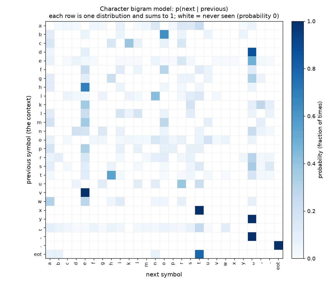
Each row of the picture is one probability distribution over the next symbol, so each row adds up to 1. The last row says how notes begin: 11 of the 14 notes start with "t".
Step 2 — one next-symbol distribution, and dependence¶
The letter "t" is followed by something 104 times. The five most likely next symbols:
| next symbol | count | \(p(\text{next} \mid \text{t})\) |
|---|---|---|
| h | 57 | 0.548 |
| ␣ | 18 | 0.173 |
| e | 12 | 0.115 |
| s | 4 | 0.038 |
| a | 2 | 0.019 |
Twelve different symbols ever follow "t".
Now compare with the overall frequency of "h". Ignoring context, "h" is the next symbol in 7.3 % of all predictions. After "t" it is 54.8 % — 7.5 times more likely. So the next symbol depends on the previous one. Symbols in text are not independent.
Step 3 — the chain rule on "the␣"¶
What probability does the model give to a note that starts with "the␣"? The first symbol is predicted from <eot>,
the second from "t", and so on:
| factor | fraction | probability | surprisal (bits) | running product |
|---|---|---|---|---|
| \(p(\text{t} \mid \text{eot})\) | 11/14 | 0.7857 | 0.348 | 0.7857 |
| \(p(\text{h} \mid \text{t})\) | 57/104 | 0.5481 | 0.868 | 0.4306 |
| \(p(\text{e} \mid \text{h})\) | 53/77 | 0.6883 | 0.539 | 0.2964 |
| \(p(\text{␣} \mid \text{e})\) | 63/130 | 0.4846 | 1.045 | 0.1436 |
The product is \(27{,}189/189{,}280 = 0.1436\). The surprisals add up to 2.799 bits, and \(2^{-2.799} = 0.1436\). The two routes agree, as the log form of the chain rule promises.
Is 0.1436 right? In the corpus, 9 of the 14 notes start with "the␣": a fraction of 0.6429. The model is far too low.
The reason is its one-symbol memory. To predict the symbol after the first "t", it uses the statistics of every "t"
in the text — in "at", "boats", "west" — not just of a "t" at the start of a note. A model with a longer context
window could use the fact that the symbol two places back was <eot>.
Treating the symbols as independent would be much worse still. Multiplying the four overall frequencies gives 0.000158.
Step 4 — whole texts, and why we add logarithms¶
The shortest note is "the next morning the fog was back, thicker than the day before." With its closing <eot> that
is 64 predictions. The model gives the whole note probability \(2^{-167.1} = 5.16\times10^{-51}\). That is 2.610 bits
per symbol.
The whole corpus has 1,056 predictions. Multiplying all 1,056 probabilities directly in float64 (the computer's standard 64-bit format for real numbers; float32 is the 32-bit one) gives exactly 0.0: the product is too small for the computer to store. Adding the surprisals instead gives 2,840.4 bits, or 2.690 bits per symbol. This is why language models are always scored with sums of logarithms, never with raw products.
How good is 2.690 bits per symbol? Compare three models on the same 1,056 predictions:
| model | bits per symbol |
|---|---|
| uniform guessing over 27 symbols (\(\log_2 27\)) | 4.755 |
| symbol frequencies, ignoring the context | 4.071 |
| bigram (one symbol of context) | 2.690 |
Each step of extra knowledge lowers the cost. Using context is what makes the bigram model good.
Finally, a sentence that never appeared: "the boats sank." It contains the pair "nk", which the corpus never has. The model gives that pair probability 0, so the sentence gets probability 0.0 and surprisal \(\infty\) (infinite) bits. One unseen pair destroys the whole score. Chapter 16 shows how the paper prevents this.
Going deeper: counting is the best possible bigram model
MY EXPLANATION Claim. Among all bigram models, the counting model gives the training text the highest probability, equivalently the lowest total surprisal.
Setup. Let \(n_{ab}\) be the number of times symbol \(b\) follows symbol \(a\) in the training text, and \(n_a = \sum_b n_{ab}\). Take any bigram model \(q(b \mid a)\). By the chain rule, the probability of the training text is a product with one factor per prediction. The factor \(q(b \mid a)\) appears exactly \(n_{ab}\) times, so the log-probability (in nats) is
Different contexts \(a\) use different distributions \(q(\cdot \mid a)\), so we can maximise each inner sum on its own. Fix \(a\) and write \(q_b = q(b \mid a)\) and \(p_b = n_{ab}/n_a\) (the counting model). We must show that \(F(q) = \sum_b n_{ab} \ln q_b\) is largest at \(q = p\).
Proof. If \(q_b = 0\) for some \(b\) with \(n_{ab} > 0\), then \(F(q) = -\infty\), which is not a maximum. Otherwise only the \(b\) with \(p_b > 0\) contribute, and
The first inequality is \(\ln x \le x - 1\) (Chapter 3). The last one holds because the \(q_b\) over some of the symbols add up to at most 1. Equality in \(\ln x \le x - 1\) needs \(q_b = p_b\) for every \(b\) with \(p_b > 0\); those \(q_b\) then add up to 1, which forces \(q_b = 0\) for the rest. So \(q = p\) is the unique maximiser. \(\blacksquare\)
Units. The proof used ln (nats). Dividing by \(\ln 2\) turns every term into bits and does not move the maximum. In our corpus the best achievable total is 2,840.4 bits.
Meaning. "Make the training text as probable as possible" is exactly the next-token-prediction objective. For a bigram model the answer is a formula: count. A neural language model aims at the same objective but has no formula; it is improved step by step (Chapter 7). The objective only concerns the training text: the best training score here still gives probability 0 to "the boats sank." This is the gap between training and fresh data that Chapter 2 warned about.
Step 5 — logits and softmax on real numbers¶
Take the context "t" and define logits as \(z = \ln(\text{count})\), with \(-\infty\) for the pairs never seen. The largest logit is \(\ln 57 = 4.043\).
- Softmax of these logits gives back the counting probabilities, up to a difference of \(1.1\times10^{-16}\) (rounding noise).
- Adding 100 to every logit changes the softmax by at most \(1.6\times10^{-15}\): shift invariance.
- Adding 1,000 to every logit breaks the naive formula: \(e\) to a power above 1,000 is too large for the computer, and 12 entries come out as "nan" (not a number). The version that first subtracts the largest logit is correct to \(9.8\times10^{-15}\).
- In float64, \(e^x\) rounds to exactly 0 for \(x\) below \(-745.13\); in float32, below \(-103.97\).
Step 6 — temperature¶
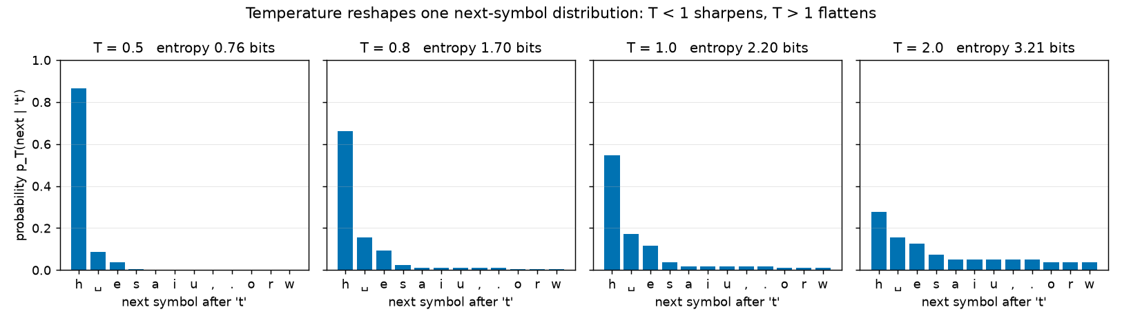
Here is the distribution after "t" at four temperatures. Its entropy is the average surprisal of a drawn symbol, \(\sum p \log_2(1/p)\) in bits: 0 for a sure thing, larger for a more spread-out distribution (Chapter 22 makes it precise).
| \(T\) | \(p_T(\text{h})\) | \(p_T(\text{e})\) | \(p_T(\text{␣})\) | entropy (bits) |
|---|---|---|---|---|
| 0.5 | 0.865 | 0.038 | 0.086 | 0.762 |
| 0.8 | 0.662 | 0.094 | 0.157 | 1.697 |
| 1.0 | 0.548 | 0.115 | 0.173 | 2.195 |
| 2.0 | 0.276 | 0.127 | 0.155 | 3.213 |
At \(T = 0.8\), the paper's sampling temperature, "h" gains probability and the entropy drops from 2.195 to 1.697 bits. At \(T = 2\) the distribution is much flatter. As \(T \to 0\), everything goes to "h" (entropy 0). As \(T \to \infty\), the 12 symbols seen after "t" become equally likely: entropy \(\log_2 12 = 3.585\) bits.
Step 7 — writing text¶
Starting after <eot>, the script samples 200 symbols at two temperatures (seed 0; | marks <eot>):
T = 0.8:  thacowe t tate crsstefothe.|the bope wrninine foftshed bound fe ind
           nd we sth we s the wat wat, by the was wathate s.|tes were fery th
          e ththe the atheapass wate oo the the, d tht t he the the scrsat t

T = 2.0:  newarr.|t cke bove t, acrssewextoud d m, wrours.|the.|thtext hrengs
          cke text.|n.|t un shrrbocksopa r urast n wed sopashe oowashewel.|ta
          f treras pochil.|ary g ule ookeare.|nge ppamonde, t in r s uthrbon
Neither looks like English — a one-symbol memory is far too short. But the lower temperature produces more real words. Over 20,000 sampled symbols at each temperature (seed 1), the share of generated words that occur in the training text is 0.164 at \(T = 0.8\), 0.092 at \(T = 1\), and 0.036 at \(T = 2\).
Greedy decoding from <eot> produces "the the the the …" forever. After "␣" the most likely symbol is "t", after "t"
it is "h", after "h" it is "e", and after "e" it is "␣". The loop closes.
Greedy decoding also misses better sequences. After "k", the most likely next symbol is "e" (4/11), and after "e" the most likely is "␣" (63/130). That two-step path has probability 0.176. But the path ",␣" has probability \(3/11 \times 1 = 0.273\): its first step is less likely, but its second step is certain.
Step 8 — byte-pair encoding on the paragraph¶
The script runs 10 BPE merges on the notes (merges do not cross note boundaries; ties go to the pair that appears first):
| merge | new token | count |
|---|---|---|
| 1 | e + ␣ → e␣ | 63 |
| 2 | t + h → th | 57 |
| 3 | th + e␣ → the␣ | 42 |
| 4 | ␣ + the␣ → ␣the␣ | 31 |
| 5 | e + r → er | 20 |
| 6 | t + ␣ → t␣ | 16 |
| 7 | s + ␣ → s␣ | 16 |
| 8 | i + n → in | 15 |
| 9 | b + o → bo | 12 |
| 10 | , + ␣ → ,␣ | 12 |
The word "the" becomes one token after three merges. The vocabulary grows from 26 to 36 symbols (not
counting <eot>). The text shrinks from 1,042 characters to 758 tokens, 1.37 characters per token. The first note now
begins [the␣] [f] [o] [g] [␣] [s] [a] [t␣] [o] [n] [␣the␣] [h] [a] [r] [bo] [u] [r] ….
Step 9 — the same ideas at GPT-2's scale¶
SOURCE: GPT-2 tokenizer GPT-2's vocabulary has \(256 + 50{,}000 + 1 = 50{,}257\) tokens, with ids 0 to 50,256.
MY EXPLANATION Those ids fit in 16 bits, since \(2^{16} = 65{,}536\). Uniform guessing over this vocabulary costs \(\log_2 50{,}257 = 15.617\) bits per token.
PAPER Table 1, p. 6 The paper's random-guess entry is 15.62; the difference, \(-0.003\), is rounding.
MY EXPLANATION A token-level bigram table for this vocabulary would need \(V^2 = 2{,}525{,}766{,}049\) numbers. That is 20.4 times the 124 million parameters of GPT-2 small (App. E), and it would still see only one token of context. A neural network instead computes the 50,257 logits for each position from up to 1,024 previous tokens, with one shared set of parameters (Chapter 5).
[SOURCE: nanoGPT prepare.py] OpenWebText's average document has 1,128.1 tokens, longer than GPT-2's
1,024-token context window.
Going deeper¶
Everything in this section is MY EXPLANATION.
The deeper blocks of this chapter sit next to the text they support:
- "Byte-pair encoding precisely, and GPT-2's version" — under Byte-pair encoding.
- "Proof of the chain rule" and "Next-token distributions always define a valid distribution, and why the end-of-text token is needed" — under The chain rule of probability.
- "Properties of softmax, with proofs" and "Softmax inside a computer" — under Logits and softmax.
- "How the paper handles documents longer than the window" — under The context window.
- "Temperature — its limits, and why it raises the entropy" — under Generating text.
- "Counting is the best possible bigram model" — in Step 4 of the worked example.
Together they prove every mathematical statement of the main text: the chain rule (with its edge cases), that a model of next-token probabilities is a model of whole documents, the five properties of softmax, the bounds on a token's surprisal in terms of its logit gap, the effect of temperature, and why counting trains the best bigram model.
Common misconceptions¶
- Misconception: a token is a word. — Actually: a token is whatever piece of text the tokenizer chose: a common word with its leading space, part of a rarer word, a single byte, or punctuation. In our 10-merge toy, "the␣" is one token but "harbour" is still six.
- Misconception: multiplying probabilities along a document assumes the tokens are independent. — Actually: the chain rule holds for every distribution. Independence would mean replacing each \(p(x_i \mid x_{<i})\) by \(p(x_i)\), which is badly wrong for text (0.000158 instead of 0.1436 in Step 3). The paper's independence assumption is about whole documents, not tokens (Chapter 15).
- Misconception: a language model stores a table of next-token probabilities. — Actually: it computes them from the context with a neural network. Even a one-token-context table for GPT-2's vocabulary would need about 2.5 billion numbers, 20.4 times the size of GPT-2 small.
- Misconception: the paper's temperature of 0.8 is part of the model that the bound certifies. — Actually: temperature is used only to generate the sample texts of Tables 6 and 7 (App. F). The bounds use the model's ordinary probabilities (\(T = 1\)), smoothed as in Chapter 16.
- Misconception: since softmax never outputs exactly 0, a language model's loss on a token is limited. — Actually: the probability is never 0 in exact arithmetic, but it can be arbitrarily small. The surprisal is at least the logit gap divided by \(\ln 2\), so it has no ceiling. In a computer it can even round to exactly 0.
- Misconception: greedy decoding finds the most probable text. — Actually: it picks the best token one step at a time. In Step 7 it picks a two-symbol path of probability 0.176 when one of 0.273 exists, and it loops forever on "the␣".
- Misconception: "bits per token" means the same thing for any model. — Actually: it depends on the tokenizer. Suppose two models give a text the same total surprisal. If one model's tokenizer cuts the text into fewer, longer tokens, that model reports more bits per token. Comparisons in bits per token are fair only with the same tokenizer, as in the paper, which uses GPT-2's throughout.
Self-test¶
Q1. Using the worked example's bigram model, what probability does it give to a note starting with "the" (without the following space)? Give the answer as a probability and as a surprisal in bits. Why is it larger than the probability of "the␣"?
Answer
By the chain rule it is the product of the first three factors of Step 3: \(p(\text{t} \mid \text{eot})\, p(\text{h} \mid \text{t})\, p(\text{e} \mid \text{h}) = (11/14)(57/104)(53/77)\). The running-product column gives 0.2964, which is \(2^{-1.754}\), so the surprisal is 1.754 bits (the sum \(0.348 + 0.868 + 0.539\) of the rounded surprisals). It is larger than 0.1436 for "the␣" because that probability multiplies in one more factor, \(p(\text{␣} \mid \text{e}) = 0.4846\), which is less than 1. Adding a token can never raise the probability of a prefix, and it never lowers the surprisal.
Q2. A friend says: "The paper writes \(p_h(X) = \prod_i p_h(x_i \mid x_{<i})\), a product over tokens. So the paper assumes tokens are independent, which is false for text." What is wrong with this, and what does the paper actually assume to be independent?
Answer
The product is the chain rule, which holds for every probability distribution over sequences; its proof uses only the definition of conditional probability. Each factor is conditioned on all earlier tokens, so the dependence between tokens is built in. Independence would mean dropping the conditioning, \(p(x_i \mid x_{<i}) = p(x_i)\), which the formula does not do. What the paper assumes independent are whole documents, drawn independently from the data source. Its loss on each document is computed from the chain-rule product (Chapter 15).
Q3. In a GPT-2 model (\(V = 50{,}257\)), the token that actually came next has a logit 20 below the largest logit at that position. Between which two values must its surprisal lie, in bits? What does this tell you about whether the per-token loss of a language model is bounded?
Answer
From the log-sum-exp bounds, the surprisal lies between \(g/\ln 2\) and \(g/\ln 2 + \log_2 V\), where \(g = 20\) is the logit gap (in nats, since logits are exponentiated with base \(e\)). That is between 28.85 and \(28.85 + 15.617 = 44.47\) bits. The lower limit \(g/\ln 2\) grows without limit as the gap grows, and nothing in an ordinary network caps the gap. So the per-token loss has no upper bound. A bound built from Hoeffding's inequality needs a loss inside a fixed interval, which is why the paper introduces prediction smoothing (Chapter 16).
Code for this chapter¶
Run it from the project root:
.venv/Scripts/python explainer/code/ch04_bigram_lm.py
Source: ch04_bigram_lm.py
"""Chapter 4 demo: a character-level bigram language model, built by counting.

Claims illustrated (all [MY EXPLANATION] unless noted):
  [1] A tiny corpus (an original paragraph, split into 14 one-sentence "notes" = tiny documents,
      each closed by an end-of-text symbol) and its vocabulary.
  [2] Next-symbol distribution p(next | 't'): top 5. Symbols in text are NOT independent:
      Pr(next = 'h') overall vs Pr(next = 'h' | previous = 't').
  [3] Chain rule: p("the " at the start of a note) as a product of 4 conditionals and as a sum of
      surprisals in bits; comparison with the (wrong) independence product.
  [4] Whole texts: probability of one note; the whole corpus underflows to 0.0 as a direct product in
      float64 but its log2 sum is finite; bits per symbol for uniform guessing, context-free symbol
      frequencies, and the bigram; a string containing an unseen pair gets probability 0.
  [5] Logits and softmax: softmax(ln counts) reproduces the counts; shift invariance; overflow of
      the naive formula; underflow thresholds of exp in float64 / float32; surprisal range for a
      token whose logit is 20 below the largest, with V = 50,257.
  [6] Temperature: entropy (bits) of p(next | 't') at T = 0.5, 0.8, 1, 2 (0.8 is the paper's
      generation temperature, [PAPER App. F, p. 17]); limits T -> 0 and T -> infinity; entropy rises with T.
  [7] Sampling 200 symbols at T = 0.8 and T = 2.0 (seed 0); share of real words (seed 1); greedy
      (argmax) decoding loops; greedy is not the most probable 2-symbol continuation.
  [8] Toy byte-pair encoding: 10 merges on the corpus.
  [9] GPT-2 numbers: V = 256 + 50,000 + 1 = 50,257 [SOURCE: GPT-2 tokenizer]; log2 V vs the paper's
      15.62 [PAPER Table 1]; size of a token-bigram table vs 124M parameters [PAPER App. E];
      average OpenWebText document length vs the 1,024-token context [SOURCE: nanoGPT prepare.py].

Writes outputs/ch04_bigram_lm.txt and docs/assets/fig/ch04_bigram_heatmap.png,
docs/assets/fig/ch04_temperature.png. Runtime: about 2 seconds. Deterministic (seed 0).
"""
import math
import sys
from fractions import Fraction
from pathlib import Path

import numpy as np

HERE = Path(__file__).resolve().parent
sys.path.insert(0, str(HERE))
import pacbound  # noqa: E402

import matplotlib  # noqa: E402
matplotlib.use("Agg")
import matplotlib.pyplot as plt  # noqa: E402

OUT_TXT = HERE / "outputs" / "ch04_bigram_lm.txt"
FIG_DIR = HERE.parent / "docs" / "assets" / "fig"
FIG_HEAT = FIG_DIR / "ch04_bigram_heatmap.png"
FIG_TEMP = FIG_DIR / "ch04_temperature.png"
OUT_TXT.parent.mkdir(parents=True, exist_ok=True)
FIG_DIR.mkdir(parents=True, exist_ok=True)

lines = []


def out(s=""):
    lines.append(s)


# ----------------------------------------------------------------- corpus
# An original paragraph (written for this explainer). Each sentence is one "note" = one tiny document.
NOTES = [
    "the fog sat on the harbour until nine, and the boats waited at the pier.",
    "the ferry left at ten with three passengers, two bikes and a crate of pears.",
    "at noon the wind turned to the west and the sea grew rough near the rocks.",
    "the gulls followed the fishing boats home and fought over the scraps.",
    "the harbour master wrote the weather in her book, then she checked the ropes.",
    "there was rain in the afternoon, so the cafe on the corner was full.",
    "the tea there is strong, the bread is warm, and the owner talks about the weather.",
    "the ferry came back at five, late but safe, with the same three passengers.",
    "by evening the sea was flat again and the light on the point turned on.",
    "the night was clear, the stars were out, and the boats rested at their moorings.",
    "then the tide went out, the mud shone under the moon, and the harbour slept.",
    "the next morning the fog was back, thicker than the day before.",
    "the boats waited again, and the harbour master wrote the same line in her book.",
    "nothing else happened that week, which is how the people of the harbour like it.",
]
EOT = "|"          # our end-of-text symbol (GPT-2's is the token <|endoftext|>)
SP = "␣"      # visible space for tables


def show(c):
    return {" ": SP, EOT: "<eot>"}.get(c, c)


letters = sorted(set("".join(NOTES)) - {" ", ",", "."})
SYMS = letters + [" ", ",", ".", EOT]
IDX = {c: i for i, c in enumerate(SYMS)}
V_TOY = len(SYMS)
n_chars = sum(len(s) for s in NOTES)
n_words = sum(len(s.split()) for s in NOTES)

# counts N[a, b] = number of times symbol b follows symbol a; every note is wrapped as <eot> note <eot>
N = np.zeros((V_TOY, V_TOY), dtype=np.int64)
for s in NOTES:
    seq = EOT + s + EOT
    for a, b in zip(seq[:-1], seq[1:]):
        N[IDX[a], IDX[b]] += 1
ROW = N.sum(axis=1)
P = N / ROW[:, None]                       # every symbol occurs as a context at least once
assert np.all(ROW > 0) and np.allclose(P.sum(axis=1), 1.0)
n_pred = int(N.sum())                      # number of predictions = chars + one closing <eot> per note
assert n_pred == n_chars + len(NOTES)

out("Chapter 4 demo: character bigram language model (ch04_bigram_lm.py, seed 0)")
out(f"[1] Corpus: {len(NOTES)} notes (tiny documents), {n_words} words, {n_chars:,} characters; "
    f"{n_pred:,} next-symbol predictions")
out(f"    vocabulary V_toy = {V_TOY} symbols: {len(letters)} letters, space, comma, period, <eot>; "
    f"table has {V_TOY}x{V_TOY} = {V_TOY * V_TOY} entries, {int((N > 0).sum())} non-zero")


def p_frac(a, b):
    return Fraction(int(N[IDX[a], IDX[b]]), int(ROW[IDX[a]]))


# ------------------------------------------------------- [2] p(next | 't')
t = IDX["t"]
order_t = np.argsort(-N[t], kind="stable")
top5 = [(SYMS[j], int(N[t, j]), P[t, j]) for j in order_t[:5]]
out(f"[2] p(next | 't'), top 5 of {int((N[t] > 0).sum())} possible next symbols "
    f"('t' is followed by something {ROW[t]} times):")
out("    " + "   ".join(f"{show(c)} {k}/{ROW[t]} = {p:.3f}" for c, k, p in top5))
marg = N.sum(axis=0) / n_pred              # how often each symbol is the next symbol, ignoring context
h = IDX["h"]
out(f"    dependence: Pr(next = 'h') = {marg[h]:.3f} overall, but Pr(next = 'h' | previous = 't') = "
    f"{P[t, h]:.3f} ({P[t, h] / marg[h]:.1f}x larger)")

# ------------------------------------------------------- [3] chain rule
word = "the "
ctx = [EOT] + list(word[:-1])
out(f"[3] Chain rule: probability that a note starts with \"the{SP}\" (context of the first symbol = <eot>)")
prod_exact = Fraction(1)
bits_sum = 0.0
indep = 1.0
for a, b in zip(ctx, word):
    f = p_frac(a, b)
    prod_exact *= f
    bits = -math.log2(float(f))
    bits_sum += bits
    indep *= marg[IDX[b]]
    out(f"    p({show(b)} | {show(a)}) = {f.numerator:>2}/{f.denominator:<3} = {float(f):.4f}"
        f"   surprisal -log2 = {bits:.3f} bits   running product {float(prod_exact):.4f}"
        f" = 2^-{bits_sum:.3f}")
prod = float(prod_exact)
assert abs(2.0 ** (-bits_sum) - prod) < 1e-12
out(f"    product = {prod_exact} = {prod:.4f};  sum of surprisals = {bits_sum:.3f} bits;  "
    f"2^-{bits_sum:.3f} = {2.0 ** -bits_sum:.4f}")
first_the = sum(s.startswith("the ") for s in NOTES)
out(f"    (in the corpus {first_the} of {len(NOTES)} notes start with \"the{SP}\" = {first_the / len(NOTES):.4f}; "
    f"if symbols were independent: {indep:.6f})")


# ------------------------------------------------------- [4] whole texts
def logp2(text_with_eots):
    """log2 probability of a symbol sequence, conditioning each symbol on the previous one."""
    tot = 0.0
    for a, b in zip(text_with_eots[:-1], text_with_eots[1:]):
        p = P[IDX[a], IDX[b]]
        if p == 0.0:
            return -math.inf
        tot += math.log2(p)
    return tot


short = min(NOTES, key=len)
lp = logp2(EOT + short + EOT)
L_short = len(short) + 1
out(f"[4] Note \"{short}\" ({L_short} predictions incl. closing <eot>):")
out(f"    p = 2^{lp:.1f} = {2.0 ** lp:.2e};  {-lp / L_short:.3f} bits per symbol")
all_probs = []
for s in NOTES:
    seq = EOT + s + EOT
    all_probs += [P[IDX[a], IDX[b]] for a, b in zip(seq[:-1], seq[1:])]
all_probs = np.array(all_probs)
direct = 1.0
for p in all_probs:
    direct *= float(p)
tot_bits = float(-np.log2(all_probs).sum())
assert direct == 0.0
out(f"    whole corpus ({len(all_probs):,} predictions): direct product in float64 = {direct} (underflow); "
    f"sum of surprisals = {tot_bits:,.1f} bits = {tot_bits / len(all_probs):.3f} bits per symbol")
uni_bits = 0.0                              # same predictions, but ignoring the context (independent symbols)
for s in NOTES:
    uni_bits += sum(-math.log2(marg[IDX[b]]) for b in s + EOT)
out(f"    bits per symbol on the corpus: uniform guess log2 {V_TOY} = {math.log2(V_TOY):.3f}; "
    f"context ignored (symbol frequencies) = {uni_bits / n_pred:.3f}; bigram = {tot_bits / n_pred:.3f}")
novel = "the boats sank."
bad = [(a, b) for a, b in zip(novel[:-1], novel[1:]) if N[IDX[a], IDX[b]] == 0]
assert bad
out(f"    unseen pair: \"{novel}\" contains {', '.join(show(a) + show(b) for a, b in bad)} "
    f"(count 0) -> p = {2.0 ** logp2(EOT + novel + EOT)}, surprisal = {-logp2(EOT + novel + EOT)} bits")


# ------------------------------------------------------- [5] logits and softmax
def softmax(z):
    z = np.asarray(z, dtype=float)
    m = np.max(z[np.isfinite(z)])
    e = np.exp(z - m)                      # exp(-inf) = 0 exactly; largest term is exp(0) = 1
    return e / e.sum()


logits_t = np.full(V_TOY, -np.inf)
logits_t[N[t] > 0] = np.log(N[t][N[t] > 0])
d0 = float(np.max(np.abs(softmax(logits_t) - P[t])))
d1 = float(np.max(np.abs(softmax(logits_t + 100.0) - softmax(logits_t))))
with np.errstate(over="ignore", invalid="ignore"):
    big = logits_t + 1000.0
    naive = np.exp(big) / np.exp(big).sum()
n_nan = int(np.isnan(naive).sum())
d2 = float(np.max(np.abs(softmax(big) - P[t])))
assert d0 < 1e-12 and d1 < 1e-12 and d2 < 1e-12 and n_nan > 0
out(f"[5] Logits for context 't': z = ln(count) (-inf where count = 0); largest z = ln {N[t].max()} "
    f"= {logits_t.max():.3f}")
out(f"    max |softmax(z) - p(.|t)| = {d0:.1e};  max |softmax(z + 100) - softmax(z)| = {d1:.1e}")
out(f"    z + 1000: naive exp overflows to inf -> {n_nan} entries are nan; subtract-the-max version: "
    f"max error {d2:.1e}")


def underflow_threshold(dtype):
    lo, hi = -2000.0, 0.0                  # exp(lo) == 0, exp(hi) > 0
    for _ in range(200):
        mid = 0.5 * (lo + hi)
        if np.exp(dtype(mid)) == 0:
            lo = mid
        else:
            hi = mid
    return hi


thr64, thr32 = underflow_threshold(np.float64), underflow_threshold(np.float32)
sm64 = softmax(np.array([0.0, -800.0]))
logsm = -800.0 - math.log1p(math.exp(-800.0))          # log-softmax of the second entry, in nats
sm32 = np.exp(np.float32(-110.0)) / (np.float32(1.0) + np.exp(np.float32(-110.0)))
assert sm64[1] == 0.0 and sm32 == 0.0
out(f"    exp(x) rounds to exactly 0 for x below {thr64:.2f} (float64) and {thr32:.2f} (float32)")
out(f"    float64: softmax([0, -800]) = [{sm64[0]:.0f}, {sm64[1]}], yet log-softmax of entry 2 = {logsm:.0f} nats "
    f"= {pacbound.nats_to_bits(logsm):.1f} bits (finite)")
out(f"    float32: softmax([0, -110]) entry 2 = {float(sm32)}")
gap = 20.0                                  # logit of a token 20 nats below the largest logit
lo_b = gap / math.log(2)
hi_b = lo_b + math.log2(pacbound.V_GPT2)
out(f"    logit gap {gap:.0f} below the largest, V = {pacbound.V_GPT2:,}: surprisal between "
    f"{gap:.0f}/ln 2 = {lo_b:.2f} and {lo_b:.2f} + log2 V = {hi_b:.2f} bits")


# ------------------------------------------------------- [6] temperature
def entropy_bits(p):
    p = p[p > 0]
    return float(-(p * np.log2(p)).sum())


def temp_dist(row_counts, T):
    z = np.full(len(row_counts), -np.inf)
    z[row_counts > 0] = np.log(row_counts[row_counts > 0])
    return softmax(z / T)


TS = [0.5, 0.8, 1.0, 2.0]
out("[6] Temperature on p(next | 't'):  p_T = softmax(z / T)")
out("      T    p_T(h)  p_T(e)  p_T(" + SP + ")   entropy (bits)")
ent_T = {}
for T in TS:
    pT = temp_dist(N[t], T)
    ent_T[T] = entropy_bits(pT)
    out(f"    {T:4.1f}   {pT[h]:.3f}   {pT[IDX['e']]:.3f}   {pT[IDX[' ']]:.3f}    {ent_T[T]:.3f}")
k_succ = int((N[t] > 0).sum())
grid = np.linspace(0.05, 20.0, 400)
ents = np.array([entropy_bits(temp_dist(N[t], T)) for T in grid])
assert np.all(np.diff(ents) > 0)
assert abs(entropy_bits(temp_dist(N[t], 1e-3)) - 0.0) < 1e-9
out(f"    T -> 0: all mass on 'h' (entropy 0, greedy);  T -> inf: uniform over the {k_succ} seen successors, "
    f"entropy log2 {k_succ} = {math.log2(k_succ):.3f} bits")
out(f"    entropy increases with T at all {len(grid)} grid points in [0.05, 20]: "
    f"{ents[0]:.3f} -> {ents[-1]:.3f} bits")


# ------------------------------------------------------- [7] sampling
def sample(T, n, rng, start=EOT):
    PT = np.array([temp_dist(N[i], T) for i in range(V_TOY)])
    cur, outc = IDX[start], []
    for _ in range(n):
        cur = int(rng.choice(V_TOY, p=PT[cur]))
        outc.append(SYMS[cur])
    return "".join(outc)


train_words = set(w.strip(",.") for s in NOTES for w in s.split())


def real_word_frac(text):
    ws = [w.strip(",.") for w in text.replace(EOT, " ").split()]
    ws = [w for w in ws if w]
    return sum(w in train_words for w in ws) / len(ws), len(ws)


out(f"[7] Samples of 200 symbols starting after <eot>, seed 0 ('|' = <eot>)")
rng = np.random.default_rng(0)
for T in (0.8, 2.0):
    smp = sample(T, 200, rng)
    out(f"    T = {T}:")
    for k in range(0, 200, 67):
        out("      " + smp[k:k + 67])
fr = {}
for T in (0.8, 1.0, 2.0):
    fr[T] = real_word_frac(sample(T, 20000, np.random.default_rng(1)))
assert fr[0.8][0] > fr[1.0][0] > fr[2.0][0]
out("    share of generated words that are words of the training text (20,000 symbols each, seed 1): "
    + ", ".join(f"T = {T}: {fr[T][0]:.3f}" for T in (0.8, 1.0, 2.0)))
cur, greedy = IDX[EOT], []
for _ in range(60):
    cur = int(np.argmax(P[cur]))
    greedy.append(SYMS[cur])
greedy = "".join(greedy)
out(f"    greedy (argmax) decoding, 60 symbols: \"{greedy}\"")
k_ = IDX["k"]                               # greedy vs the most probable 2-symbol continuation after 'k'
g1 = int(np.argmax(P[k_]))
g2 = int(np.argmax(P[g1]))
two = P[k_][:, None] * P                    # two[b, c] = p(b | k) p(c | b)
b1, b2 = np.unravel_index(int(np.argmax(two)), two.shape)
assert two[b1, b2] > P[k_, g1] * P[g1, g2]
out(f"    after 'k': greedy takes '{show(SYMS[g1])}' ({p_frac('k', SYMS[g1])}) then '{show(SYMS[g2])}' "
    f"({p_frac(SYMS[g1], SYMS[g2])}) -> {P[k_, g1] * P[g1, g2]:.3f}; best pair '{show(SYMS[b1])}{show(SYMS[b2])}' "
    f"= {p_frac('k', SYMS[b1])} x {p_frac(SYMS[b1], SYMS[b2])} = {two[b1, b2]:.3f}")


# ------------------------------------------------------- [8] toy BPE
def bpe(notes, n_merges):
    toks = [list(s) for s in notes]       # merges never cross note boundaries
    merges = []
    for _ in range(n_merges):
        count, first, pos = {}, {}, 0
        for tl in toks:
            for a, b in zip(tl[:-1], tl[1:]):
                count[(a, b)] = count.get((a, b), 0) + 1
                first.setdefault((a, b), pos)
                pos += 1
            pos += 1
        best = max(count, key=lambda pr: (count[pr], -first[pr]))   # most frequent; tie -> earliest
        merges.append((best, count[best]))
        new = []
        for tl in toks:
            res, i = [], 0
            while i < len(tl):
                if i + 1 < len(tl) and (tl[i], tl[i + 1]) == best:
                    res.append(tl[i] + tl[i + 1])
                    i += 2
                else:
                    res.append(tl[i])
                    i += 1
            new.append(res)
        toks = new
    return merges, toks


merges, toks = bpe(NOTES, 10)
n_tok = sum(len(tl) for tl in toks)
out("[8] Toy byte-pair encoding: 10 merges (pair count shown; most frequent pair first, ties -> earliest)")
def vis(tok):
    return tok.replace(" ", SP)


for k in range(0, 10, 2):
    out("    " + "     ".join(f"{k + j + 1:>2}. '{vis(a)}' + '{vis(b)}' -> '{vis(a + b)}'  (count {c})"
                            for j, ((a, b), c) in enumerate(merges[k:k + 2])))
out(f"    corpus length: {n_chars:,} characters -> {n_tok:,} tokens ({n_chars / n_tok:.2f} characters per token); "
    f"vocabulary {V_TOY - 1} + 10 = {V_TOY - 1 + 10} (without <eot>)")
out("    note 1 as tokens: " + " ".join("[" + vis(tk) + "]" for tk in toks[0][:26]) + " ...")

# ------------------------------------------------------- [9] GPT-2 numbers
V = 256 + 50_000 + 1
assert V == pacbound.V_GPT2
lv = pacbound.random_guess_bpd(V)
assert round(lv, 2) == 15.62
out(f"[9] GPT-2: V = 256 byte tokens + 50,000 merges + 1 <|endoftext|> = {V:,}; token ids 0..{V - 1:,} "
    f"fit in 16 bits (2^16 = {2 ** 16:,})")
out(f"    log2 V = {lv:.3f} bits (paper's random-guess BPD 15.62; diff {lv - 15.62:+.3f})")
out(f"    a token-bigram table would need V^2 = {V * V:,} numbers = {V * V / 124e6:.1f} x the 124M parameters "
    f"of GPT-2 small; one logit list per position has {V:,} entries")
avg_doc = pacbound.OWT_TRAIN_TOKENS / pacbound.M_DOCS
out(f"    OpenWebText: {pacbound.OWT_TRAIN_TOKENS:,} tokens / {pacbound.M_DOCS:,} documents = {avg_doc:,.1f} "
    f"tokens per document (incl. its <|endoftext|>) > context window {pacbound.CONTEXT:,}")

# ------------------------------------------------------- figures
order = letters + [" ", ",", ".", EOT]
labels = [show(c) if c != EOT else "eot" for c in order]
fig, ax = plt.subplots(figsize=(8.6, 7.4))
cmap = matplotlib.colormaps["Blues"].copy()
cmap.set_bad("white")                      # probability exactly 0 (pair never seen) is drawn white
im = ax.imshow(np.ma.masked_equal(P, 0.0), cmap=cmap, vmin=0, vmax=1, interpolation="nearest")
ax.set_xticks(range(V_TOY))
ax.set_xticklabels(labels, fontsize=9, rotation=90)
ax.set_yticks(range(V_TOY))
ax.set_yticklabels(labels, fontsize=9)
ax.set_xlabel("next symbol", fontsize=11)
ax.set_ylabel("previous symbol (the context)", fontsize=11)
ax.set_title("Character bigram model: p(next | previous)\neach row is one distribution and sums to 1; "
             "white = never seen (probability 0)", fontsize=11)
ax.set_xticks(np.arange(-0.5, V_TOY, 1), minor=True)
ax.set_yticks(np.arange(-0.5, V_TOY, 1), minor=True)
ax.grid(which="minor", color="#e6e6e6", lw=0.4)
ax.tick_params(which="minor", length=0)
cb = fig.colorbar(im, ax=ax, fraction=0.046, pad=0.03)
cb.set_label("probability (fraction of times)", fontsize=10)
fig.tight_layout()
fig.savefig(FIG_HEAT, dpi=130)
plt.close(fig)

succ = [j for j in np.argsort(-N[t], kind="stable") if N[t, j] > 0]
fig, axes = plt.subplots(1, 4, figsize=(12.5, 3.6), sharey=True)
for ax, T in zip(axes, TS):
    pT = temp_dist(N[t], T)
    ax.bar(range(len(succ)), pT[succ], color="#0072B2", width=0.8)
    ax.set_xticks(range(len(succ)))
    ax.set_xticklabels([show(SYMS[j]) if SYMS[j] != EOT else "eot" for j in succ], fontsize=10)
    ax.set_title(f"T = {T}   entropy {ent_T[T]:.2f} bits", fontsize=11)
    ax.set_xlabel("next symbol after 't'", fontsize=10)
    ax.grid(axis="y", alpha=0.3, lw=0.6)
    ax.set_ylim(0, 1)
axes[0].set_ylabel("probability p_T(next | 't')", fontsize=10)
fig.suptitle("Temperature reshapes one next-symbol distribution: T < 1 sharpens, T > 1 flattens", fontsize=12)
fig.tight_layout()
fig.savefig(FIG_TEMP, dpi=130)
plt.close(fig)
out(f"figures: docs/assets/fig/{FIG_HEAT.name}, docs/assets/fig/{FIG_TEMP.name}. All assertions passed.")

text = "\n".join(lines) + "\n"
OUT_TXT.write_text(text, encoding="utf-8")
try:                                       # Windows consoles may not be UTF-8 (the visible space is U+2423)
    sys.stdout.reconfigure(encoding="utf-8", errors="replace")
except AttributeError:
    pass
print(text, end="")
Output:
Chapter 4 demo: character bigram language model (ch04_bigram_lm.py, seed 0)
[1] Corpus: 14 notes (tiny documents), 203 words, 1,042 characters; 1,056 next-symbol predictions
    vocabulary V_toy = 27 symbols: 23 letters, space, comma, period, <eot>; table has 27x27 = 729 entries, 214 non-zero
[2] p(next | 't'), top 5 of 12 possible next symbols ('t' is followed by something 104 times):
    h 57/104 = 0.548   ␣ 18/104 = 0.173   e 12/104 = 0.115   s 4/104 = 0.038   a 2/104 = 0.019
    dependence: Pr(next = 'h') = 0.073 overall, but Pr(next = 'h' | previous = 't') = 0.548 (7.5x larger)
[3] Chain rule: probability that a note starts with "the␣" (context of the first symbol = <eot>)
    p(t | <eot>) = 11/14  = 0.7857   surprisal -log2 = 0.348 bits   running product 0.7857 = 2^-0.348
    p(h | t) = 57/104 = 0.5481   surprisal -log2 = 0.868 bits   running product 0.4306 = 2^-1.215
    p(e | h) = 53/77  = 0.6883   surprisal -log2 = 0.539 bits   running product 0.2964 = 2^-1.754
    p(␣ | e) = 63/130 = 0.4846   surprisal -log2 = 1.045 bits   running product 0.1436 = 2^-2.799
    product = 27189/189280 = 0.1436;  sum of surprisals = 2.799 bits;  2^-2.799 = 0.1436
    (in the corpus 9 of 14 notes start with "the␣" = 0.6429; if symbols were independent: 0.000158)
[4] Note "the next morning the fog was back, thicker than the day before." (64 predictions incl. closing <eot>):
    p = 2^-167.1 = 5.16e-51;  2.610 bits per symbol
    whole corpus (1,056 predictions): direct product in float64 = 0.0 (underflow); sum of surprisals = 2,840.4 bits = 2.690 bits per symbol
    bits per symbol on the corpus: uniform guess log2 27 = 4.755; context ignored (symbol frequencies) = 4.071; bigram = 2.690
    unseen pair: "the boats sank." contains nk (count 0) -> p = 0.0, surprisal = inf bits
[5] Logits for context 't': z = ln(count) (-inf where count = 0); largest z = ln 57 = 4.043
    max |softmax(z) - p(.|t)| = 1.1e-16;  max |softmax(z + 100) - softmax(z)| = 1.6e-15
    z + 1000: naive exp overflows to inf -> 12 entries are nan; subtract-the-max version: max error 9.8e-15
    exp(x) rounds to exactly 0 for x below -745.13 (float64) and -103.97 (float32)
    float64: softmax([0, -800]) = [1, 0.0], yet log-softmax of entry 2 = -800 nats = -1154.2 bits (finite)
    float32: softmax([0, -110]) entry 2 = 0.0
    logit gap 20 below the largest, V = 50,257: surprisal between 20/ln 2 = 28.85 and 28.85 + log2 V = 44.47 bits
[6] Temperature on p(next | 't'):  p_T = softmax(z / T)
      T    p_T(h)  p_T(e)  p_T(␣)   entropy (bits)
     0.5   0.865   0.038   0.086    0.762
     0.8   0.662   0.094   0.157    1.697
     1.0   0.548   0.115   0.173    2.195
     2.0   0.276   0.127   0.155    3.213
    T -> 0: all mass on 'h' (entropy 0, greedy);  T -> inf: uniform over the 12 seen successors, entropy log2 12 = 3.585 bits
    entropy increases with T at all 400 grid points in [0.05, 20]: 0.000 -> 3.582 bits
[7] Samples of 200 symbols starting after <eot>, seed 0 ('|' = <eot>)
    T = 0.8:
      thacowe t tate crsstefothe.|the bope wrninine foftshed bound fe ind
       nd we sth we s the wat wat, by the was wathate s.|tes were fery th
      e ththe the atheapass wate oo the the, d tht t he the the scrsat t
    T = 2.0:
      newarr.|t cke bove t, acrssewextoud d m, wrours.|the.|thtext hrengs
      cke text.|n.|t un shrrbocksopa r urast n wed sopashe oowashewel.|ta
      f treras pochil.|ary g ule ookeare.|nge ppamonde, t in r s uthrbon
    share of generated words that are words of the training text (20,000 symbols each, seed 1): T = 0.8: 0.164, T = 1.0: 0.092, T = 2.0: 0.036
    greedy (argmax) decoding, 60 symbols: "the the the the the the the the the the the the the the the "
    after 'k': greedy takes 'e' (4/11) then '␣' (63/130) -> 0.176; best pair ',␣' = 3/11 x 1 = 0.273
[8] Toy byte-pair encoding: 10 merges (pair count shown; most frequent pair first, ties -> earliest)
     1. 'e' + '␣' -> 'e␣'  (count 63)      2. 't' + 'h' -> 'th'  (count 57)
     3. 'th' + 'e␣' -> 'the␣'  (count 42)      4. '␣' + 'the␣' -> '␣the␣'  (count 31)
     5. 'e' + 'r' -> 'er'  (count 20)      6. 't' + '␣' -> 't␣'  (count 16)
     7. 's' + '␣' -> 's␣'  (count 16)      8. 'i' + 'n' -> 'in'  (count 15)
     9. 'b' + 'o' -> 'bo'  (count 12)     10. ',' + '␣' -> ',␣'  (count 12)
    corpus length: 1,042 characters -> 758 tokens (1.37 characters per token); vocabulary 26 + 10 = 36 (without <eot>)
    note 1 as tokens: [the␣] [f] [o] [g] [␣] [s] [a] [t␣] [o] [n] [␣the␣] [h] [a] [r] [bo] [u] [r] [␣] [u] [n] [t] [i] [l] [␣] [n] [in] ...
[9] GPT-2: V = 256 byte tokens + 50,000 merges + 1 <|endoftext|> = 50,257; token ids 0..50,256 fit in 16 bits (2^16 = 65,536)
    log2 V = 15.617 bits (paper's random-guess BPD 15.62; diff -0.003)
    a token-bigram table would need V^2 = 2,525,766,049 numbers = 20.4 x the 124M parameters of GPT-2 small; one logit list per position has 50,257 entries
    OpenWebText: 9,035,582,198 tokens / 8,009,762 documents = 1,128.1 tokens per document (incl. its <|endoftext|>) > context window 1,024
figures: docs/assets/fig/ch04_bigram_heatmap.png, docs/assets/fig/ch04_temperature.png. All assertions passed.