21. Quantization and quantization-aware training¶

Where this fits

Prerequisites: Chapter 3 ($\log_2$, bits, the ceiling $\lceil\cdot\rceil$, the 8,192-bit kilobyte), Chapter 7 (gradient, chain rule, Adam, reparameterization, finite-difference check), Chapter 14 (compressed size $C(h)$ and why every bit counts) and Chapter 20 (SubLoRA: the only trained numbers are the $d$ subspace coordinates $w\in\mathbb R^d$). Used later by: Chapter 22 (coding the quantized weights with arithmetic coding), Chapter 24 (Algorithm 1's TRAIN_QUANTIZE) and Chapter 28 (mini replication). Purpose: explain how the paper turns $d$ real numbers into $d$ choices among a handful of allowed values, and how it trains the model so that this rounding costs little accuracy.

The problem this chapter solves¶

Everything in this section is MY EXPLANATION unless tagged.

After SubLoRA training (Chapter 20), the whole trained part of the model is one list of real numbers, the subspace coordinates $w = (w_1,\dots,w_d)$. Everything else (architecture, random start $\theta_0$, fixed initial LoRA factors $\phi_0$, random projection $P$) is rebuilt from fixed seeds and costs nothing to describe.

A computer normally stores each real number as a float32: 32 bits. For $d = 50{,}000$ coordinates that is 1,600,000 bits, or 195.31 KB, as printed by ch21_quantize.py, output [1]. (1 KB = 8,192 bits: the convention of Lotfi et al. 2022 that this explainer follows, Chapter 3, erratum E35.)

[PAPER Fig. 2 left, p. 5; read exactly from the PDF by fig_extract.py] The paper's best bits-per-token model has $d = 50{,}000$ and a compressed size of 16.5325 KB. MY EXPLANATION With 1 KB = 8,192 bits (SOURCE: Lotfi et al. 2022, erratum E35) that is 135,434 bits, or 2.709 bits per coordinate. The float32 version would be 11.8 times larger (output [1]).

The bound of Chapter 14 charges for every bit of $C(h)$. So the question is: how do we get from 32 bits per number down to under 3, without wrecking the model? The paper uses two steps:

Quantize: replace each $w_i$ by the nearest of a few allowed values (this chapter).
Entropy-code: write down which allowed value each coordinate got, spending fewer bits on values that occur often (Chapter 22).

Step 1 damages the model a little. Quantization-aware training (this chapter) repairs most of the damage by training the model while it is quantized.

Only the $d$ coordinates are quantized, never the $D$ parameters of GPT-2 itself. GPT-2 small has $D = 123{,}689{,}472$ parameters (nanoGPT count, [SOURCE: nanoGPT parameter count via pacbound.gpt2_params]), which is 2,474 times $d = 50{,}000$. Quantizing all $D$ of them at 4 bits each would cost 494.8 million bits (output [1]); the subspace trick of Chapters 18–20 is what makes the small number possible.

Intuition (and where the analogy breaks)¶

Everything in this section is MY EXPLANATION.

Think of a shop that decides every price must be one of eleven "price points". Each product's price is rounded to the nearest point. A clever shop does not space the points evenly from $0 to $1,000. It puts many points where most of its products are priced (say between $5 and $30) and only a few out in the expensive range. That keeps the rounding damage small for most products. Choosing the points this way is what k-means does.

Now go one step further. The shop knows the prices will be rounded. So it re-tunes its unrounded prices, watching the revenue that the rounded prices bring in, and it is also allowed to slide the price points themselves. That is quantization-aware training: training with the rounding in the loop.

Where it breaks:

Rounding has no slope. A shopkeeper can see that nudging a price by one cent changes revenue a little. For a rounded weight, nudging $w_i$ by a tiny amount changes nothing at all, until $w_i$ crosses a halfway point and the rounded value jumps. Calculus therefore gives a slope of exactly zero almost everywhere, and gradient descent receives no signal. The fix, the straight-through estimator, deliberately pretends that rounding is the identity when computing slopes. It works well in practice, but it is an approximation with no guarantee; we show below a tiny case where it makes things worse.
The goal is not small rounding error. The shop wants revenue, not prices close to the originals. Likewise the paper wants low training loss and few bits; small rounding error is only a proxy.

Precise definition¶

Everything in this section is MY EXPLANATION unless a paragraph carries another tag.

Levels, codebook and nearest-level assignment¶

Quantization means replacing each number by one value from a small, fixed set. The allowed values are the quantization levels $c_1, c_2, \dots, c_{L_q}$. Their list $c = (c_1,\dots,c_{L_q})$ is the codebook, and $L_q$ is the number of levels (11 or 17 in the paper).

The nearest-level assignment of coordinate $i$ is the index of the closest level:

\[ q(i) = \arg\min_{k \in \{1,\dots,L_q\}} \lvert w_i - c_k \rvert . \]

Here "$\arg\min_k$" means "the $k$ that makes the expression smallest" (ties, which almost never happen with real data, go to the smaller index). The quantized coordinate is the level it is assigned to:

\[ \hat w_i = c_{q(i)}, \qquad \hat w = (\hat w_1,\dots,\hat w_d). \]

All coordinates assigned to the same level $k$ form the cluster (also called bin) of level $k$: $S_k = \{\, i : q(i) = k \,\}$. Its size is the count $n_k = \lvert S_k\rvert$, and $n_1 + \dots + n_{L_q} = d$.

To store $\hat w$ you need the codebook ($L_q$ numbers) plus the sequence of indices $q(1),\dots,q(d)$: $d$ symbols, each from an alphabet of $L_q$ letters.

PAPER App. C, p. 15 The paper builds $\hat w$ exactly this way: each $\hat w_i$ is the level $c_q$ with $q$ the index minimizing $\lvert w_i - c_k\rvert$; the clusters $c$ are learned together with $w$ and initialized by k-means.

Paper erratum E16: what the number of levels is called

PAPER App. C, p. 15; App. E, p. 17 The paper calls the number of quantization levels $C$ in Algorithm 1's inputs (and lines 4, 9, 10), in the App. C prose and in Appendix E ("$C \in \{11, 17\}$"), but $L$ in Algorithm 1's function signature (line 2), in the codebook $c = [c_1,\dots,c_L]$ and in the closing App. C sentence ("values of $r$, $d$, $L$ and $\alpha$"). MY EXPLANATION $C$ already means the compressed size $C(h)$, and $L$ already means a document length and the context length. This explainer writes $L_q$ for the number of levels (erratum E16).

Quantization error¶

The quantization error of coordinate $i$ is $e_i = w_i - \hat w_i$. We summarize it by the mean squared error

\[ \mathrm{MSE} = \frac1d \sum_{i=1}^{d} (w_i - \hat w_i)^2 , \]

which has the units of $w$ squared. (For a Gaussian test vector we report it in units of the variance $\mathrm{sd}^2$.)

Uniform versus learned levels¶

Uniform levels are evenly spaced, e.g. $L_q$ points from the smallest to the largest $w_i$. Learned (non-uniform) levels are placed where they help; the paper starts from k-means levels, which crowd where the coordinates are dense, and then lets training move them.

k-means in one dimension (Lloyd's algorithm)¶

k-means chooses the codebook that makes the total squared error small:

\[ J(c, q) = \sum_{i=1}^{d} \big(w_i - c_{q(i)}\big)^2 . \]

Lloyd's algorithm alternates two steps until the assignment stops changing:

Assign: with the levels fixed, give every coordinate its nearest level.
Update: with the assignments fixed, move every level to the mean of its cluster, $c_k \leftarrow \frac{1}{n_k}\sum_{i \in S_k} w_i$ (an empty cluster keeps its level).

Each step can only lower $J$ or leave it unchanged, and there are only finitely many ways to assign the coordinates to levels, so the algorithm settles down after finitely many rounds. It does not always find the best codebook: it can stop at a local optimum, a codebook that neither step can improve but that is worse than another codebook.

Going deeper: proof that Lloyd's algorithm never increases the squared error, and stops

MY EXPLANATION Fix the data $w_1,\dots,w_d$. Nothing in this proof is random.

Assignment step. Hold $c$ fixed. $J(c,q)$ is a sum of $d$ separate terms, and term $i$ depends only on $q(i)$. Choosing $q(i)$ to be the nearest level makes term $i$ as small as it can be, so for the new assignment $q'$ and any old assignment $q$,

\[ J(c, q') \le J(c, q). \]

Update step. Hold $q$ fixed. $J$ splits into one sum per cluster, $J = \sum_k \sum_{i\in S_k}(w_i - c_k)^2$, and level $c_k$ appears only in its own sum. Take one cluster $S$ with $n$ members and mean $\bar w = \frac1n\sum_{i\in S} w_i$. Add and subtract $\bar w$ inside the square:

\[ \begin{aligned} \sum_{i\in S}(w_i - c)^2 &= \sum_{i\in S}\big((w_i - \bar w) + (\bar w - c)\big)^2 \\ &= \sum_{i\in S}(w_i - \bar w)^2 + 2(\bar w - c)\sum_{i\in S}(w_i - \bar w) + n(\bar w - c)^2 \\ &= \sum_{i\in S}(w_i - \bar w)^2 + n(\bar w - c)^2 . \end{aligned} \]

The middle term vanished because $\sum_{i\in S}(w_i - \bar w) = n\bar w - n\bar w = 0$. The last line is smallest exactly when $c = \bar w$, and moving $c$ to $\bar w$ lowers the cluster's error by $n(\bar w - c)^2 \ge 0$. So the update step cannot increase $J$ either.

Stopping. After an update step every non-empty cluster's level is its cluster mean, so the error after an update step, $\sum_k\sum_{i\in S_k}(w_i-\bar w_k)^2$, depends only on the assignment (empty clusters contribute nothing). Use the tie rule "keep your current level unless another level is strictly closer". Then any change of assignment strictly lowers $J$, so the post-update error strictly falls from round to round and no assignment can ever come back. There are at most $L_q^{\,d}$ assignments, a finite number, so the algorithm stops after finitely many rounds. (With continuous data ties have probability zero, so the script's simpler rule "ties go to the lower index" gives the same run.)

Why one dimension is easy. If $c_k < c_{k+1}$, a point $x$ is closer to $c_k$ exactly when $x < (c_k + c_{k+1})/2$. So each cluster is an interval between consecutive midpoints. The assignment step is a sorted search, and cluster sums come from running totals; this is how lloyd_1d in the script handles $d = 50{,}000$ quickly.

A local optimum, by hand (output [3]). Points $0,1,2,10,11,12,20,21,22$ and $L_q = 3$. Start at levels $(0, 1, 16)$. The midpoints are $0.5$ and $8.5$, so the clusters are $\{0\}$, $\{1,2\}$ and $\{10,\dots,22\}$, with means $0$, $1.5$ and $16$. The new midpoints $0.75$ and $8.75$ give the same clusters, so Lloyd's algorithm stops at $(0, 1.5, 16)$ with counts $[1, 2, 6]$. The squared error is $0 + (0.25 + 0.25) + (36+25+16+16+25+36) = 154.5$. Starting at $(1, 11, 21)$ instead gives the three natural groups and squared error $6$. Both are fixed points; only the second is the best codebook.

What the quantized vector costs in bits¶

This subsection is MY EXPLANATION unless tagged.

Writing down $\hat w$ means writing down $d$ level indices. Two prices are worth knowing.

Fixed-length code. Give every index the same number of bits. Naming one of $L_q$ things takes $\lceil \log_2 L_q \rceil$ bits (Chapter 3): 4 bits for $L_q = 11$, 5 bits for $L_q = 17$ (output [1]). These are the bits per weight before entropy coding.
Entropy limit. If level $k$ is used by a fraction $\hat p_k = n_k/d$ of the coordinates, the best possible average cost per index is the entropy $H(\hat p) = -\sum_k \hat p_k \log_2 \hat p_k$ bits, a quantity that Chapter 22 defines and proves to be the limit. Arithmetic coding, the entropy code the paper uses (a method that turns the whole index sequence into one bit string, made precise in Chapter 22), gets within 2 bits of $d\,H(\hat p)$ for the whole vector. The entropy is at most $\log_2 L_q$ (3.4594 bits for 11 levels, 4.0875 bits for 17), reached only when all levels are used equally often. Skewed usage gives fewer bits.

Two small extra costs sit on top:

The codebook. At 16 bits per level, 176 bits for $L_q = 11$ and 272 bits for $L_q = 17$ (output [1]). The decoder also needs the level counts $n_k$, about $\lceil\log_2 d\rceil$ more bits per level (Chapter 22). Whether the paper counts these is not stated (erratum E18; Chapter 22 shows the authors' code does).
The choice of $L_q$. PAPER App. E, p. 17 The paper tries $L_q \in \{11, 17\}$. MY EXPLANATION Naming one of two values costs $\log_2 2 = 1$ bit in the prior (Chapter 14).

Why rounding has no useful gradient¶

Hold the codebook fixed. As $w_i$ slides along the number line, $\hat w_i$ stays at one level, then jumps to the next level when $w_i$ passes a midpoint. Its graph is a staircase. A staircase has slope 0 on every flat step and no slope at all at the jumps. So the true derivative of the loss with respect to $w$ is zero wherever it exists:

\[ \frac{\partial \mathcal L}{\partial w_j} = \sum_{i} \frac{\partial \mathcal L}{\partial \hat w_i}\, \frac{\partial \hat w_i}{\partial w_j} = 0 \quad\text{almost everywhere}. \]

Here $\mathcal L$ is the training objective (the loss of the quantized model, Chapter 7) and "almost everywhere" means "everywhere except at the finitely many midpoints". Plain gradient descent on $w$ would never move.

Going deeper: the derivative of the nearest-level map is 0 almost everywhere

MY EXPLANATION Sort the levels, $c_1 < \dots < c_{L_q}$, and let $m_k = (c_k + c_{k+1})/2$ be the midpoints ($k = 1,\dots,L_q-1$), with $m_0 = -\infty$ and $m_{L_q} = +\infty$. By the one-dimensional argument in the Lloyd proof above, for fixed $c$

\[ \hat w_i = c_k \quad\text{whenever}\quad m_{k-1} < w_i < m_k . \]

On each open interval $(m_{k-1}, m_k)$ the function $w_i \mapsto \hat w_i$ is constant, so its derivative there is 0. At $w_i = m_k$ the value jumps by $c_{k+1} - c_k > 0$; a function that jumps is not continuous, so it has no derivative there. The set $\{m_1,\dots,m_{L_q-1}\}$ is finite and has total length zero, which is what "almost everywhere" means. Also, $\hat w_i$ does not depend on $w_j$ for $j \ne i$, so $\partial \hat w_i/\partial w_j = 0$ for $j \ne i$ everywhere.

By the chain rule (Chapter 7) every partial derivative $\partial\mathcal L/\partial w_j$ is a sum of terms each multiplied by some $\partial \hat w_i/\partial w_j = 0$, hence 0. Output [5] confirms this with a finite-difference check on a six-coordinate example: all six true derivatives print as $+0.000$.

The straight-through estimator¶

The straight-through estimator (STE) fixes the zero-gradient problem by decree. In the backward pass (the gradient computation) it pretends that rounding was the identity map:

\[ \frac{\partial \hat w_i}{\partial w_j} := \mathbf 1[i = j] \qquad\Longrightarrow\qquad \frac{\partial \mathcal L}{\partial w_i} := \frac{\partial \mathcal L}{\partial \hat w_i} . \]

The symbol $:=$ marks a definition, not a fact: the right side is a stand-in for a derivative that is really 0. The gradient is still evaluated at the quantized weights $\hat w$. Read it as: "the loss would like $\hat w_i$ to move this way; move the hidden full-precision $w_i$ that way, and once it has drifted past a midpoint, $\hat w_i$ will follow."

SOURCE: Lotfi et al. 2022, §4.2, Eq. 4 The earlier paper that this one follows defines exactly these gradients, writing $\delta_{ij}$ (1 if $i = j$, else 0) where we write $\mathbf 1[i=j]$, and $\partial \hat w_i/\partial c_k = \mathbf 1[q(i) = k]$ for the levels. MY EXPLANATION We avoid $\delta_{ij}$ because $\delta$ is this explainer's failure probability.

The levels need no pretending. Since $\hat w_i = c_{q(i)}$, a small change of $c_k$ moves exactly the coordinates in cluster $k$ by the same amount, so the codebook gradient is

\[ \frac{\partial \mathcal L}{\partial c_k} = \sum_{i:\,q(i) = k} \frac{\partial \mathcal L}{\partial \hat w_i} , \]

the sum of the loss gradients over the cluster of level $k$. This is an exact derivative (almost everywhere), not an estimate. The deep block below derives it.

Going deeper: the codebook gradient is exact

MY EXPLANATION Write the quantized coordinate with indicators:

\[ \hat w_i = \sum_{k=1}^{L_q} c_k\, \mathbf 1[q(i) = k]. \]

Suppose no $w_i$ sits exactly on a midpoint (true almost everywhere). Each assignment is decided by strict inequalities $\lvert w_i - c_{q(i)}\rvert < \lvert w_i - c_k\rvert$, and both sides change continuously with $c$. So a small enough change of $c$ leaves every $q(i)$ unchanged, and near the current $c$ the indicators are constants. Differentiating the display term by term,

\[ \frac{\partial \hat w_i}{\partial c_k} = \mathbf 1[q(i) = k]. \]

The loss depends on $c$ only through $\hat w$, so the chain rule gives

\[ \frac{\partial \mathcal L}{\partial c_k} = \sum_{i=1}^{d} \frac{\partial \mathcal L}{\partial \hat w_i}\,\mathbf 1[q(i)=k] = \sum_{i:\,q(i)=k} \frac{\partial \mathcal L}{\partial \hat w_i} . \]

Output [5] checks this numerically: for levels $(-1, 0, 1)$ the cluster sums are $+0.62912$, $+7.92535$, $+6.12764$, and central finite differences in $c$ agree to within $1.0\times10^{-9}$. Only the $w$-half of the STE is a pretence; the $c$-half is calculus.

Quantization-aware training¶

Quantization-aware training (QAT) trains with the quantizer inside the model:

Start from trained full-precision $w$; set the codebook $c$ by k-means on the entries of $w$.
Repeat for some number of steps:
- Forward pass: compute $q(i)$ and $\hat w_i = c_{q(i)}$; evaluate the loss $\mathcal L$ of the model built from $\hat w$ (not from $w$).
- Backward pass: compute $g_i = \partial\mathcal L/\partial \hat w_i$.
- Update: $w_i \leftarrow w_i - \rho\, g_i$ (STE) and $c_k \leftarrow c_k - \rho \sum_{i: q(i) = k} g_i$ (codebook gradient), with step size $\rho$; any optimizer such as Adam can replace the plain step.
Output the final $\hat w$: the codebook and the assignments. The full-precision $w$ is thrown away.

The alternative, post-training quantization, rounds once after training and stops (step 1 only).

PAPER §3, p. 4 The paper describes Lotfi et al. (2022) as using a learned quantization strategy that optimizes over the quantized weights and the quantization levels, followed by arithmetic coding with the empirical probabilities of the quantization bins. PAPER §6.1, p. 7 Near the end of training, the paper trains for additional steps with QAT "with a small number of quantization levels", then expresses $w$ in this quantization and arithmetic-codes it. PAPER App. C, Algorithm 1 lines 4 and 9–15, p. 15 Line 4 calls TRAIN_QUANTIZE on the SubLoRA vector $w$; line 10 initializes $c$ by GET_CLUSTERS; line 12 updates both $c$ and $w$ by gradient steps on $\mathcal L(w,c)$ with step size $\rho$, for quant_epochs rounds; line 14 returns $\hat w$. PAPER App. E, pp. 16–17 Appendix E calls this "aggressive learned quantization on $w$" following Lotfi et al. (2022), with $L_q \in \{11, 17\}$.

Paper erratum E17: line 12 needs the straight-through estimator, which the paper never mentions

PAPER App. C, p. 15 Line 12 differentiates the loss with respect to $w$ although the loss is computed from the nearest-level vector $\hat w$. MY EXPLANATION As shown above, that derivative is 0 almost everywhere, so a literal reading of line 12 never moves $w$. The method only works with the STE of Lotfi et al. (2022, Eq. 4). The function signature also takes an argument $L$ that is not among the listed inputs (they call the levels $C$) (erratum E17).

Paper erratum E64: TRAIN_QUANTIZE returns a vector it never computes

PAPER App. C, Algorithm 1 lines 9–15, p. 15 Lines 10–13 update only $c$ and $w$; line 14 returns $\hat w$, whose construction ($\hat w_i = c_q$ with $q = \arg\min_k\lvert w_i - c_k\rvert$) appears only in the prose below the algorithm. The step size $\rho$, the loss $\mathcal L(w,c)$ and quant_epochs are never defined (erratum E64). MY EXPLANATION Read as intended, line 14 should first apply the nearest-level assignment with the final $c$ and $w$; that is what our QAT steps above and the script do.

Going deeper: the STE has no guarantee — a one-weight example

MY EXPLANATION Output [6]. One weight, levels $\{0, 1\}$ (midpoint $0.5$), loss $\mathcal L(\hat w) = (\hat w - 0.4)^2$, plain gradient steps with step size $0.05$, start $w = 0.2$. Nothing is random. The best the quantized weight can do is $\hat w = 0$ with loss $0.4^2 = 0.16$; $\hat w = 1$ costs $0.6^2 = 0.36$.

Levels fixed. While $w < 0.5$, $\hat w = 0$ and the STE gradient is $2(0 - 0.4) = -0.8$, so each step adds $0.05 \times 0.8 = 0.04$ to $w$: the loss "wants" $\hat w$ to go up toward $0.4$. After a few steps $w$ passes $0.5$, $\hat w$ jumps to 1, the gradient becomes $2(1-0.4) = 1.2$, and each step subtracts $0.06$. So $w$ keeps crossing back and forth over the midpoint. In the long run the drifts must cancel. If a fraction $f$ of steps sit on level 1,

\[ 0.04\,(1-f) = 0.06\,f \quad\Longrightarrow\quad f = \frac{0.04}{0.10} = 0.4 , \]

and the average loss is $0.16\,(1-f) + 0.36\,f = 0.096 + 0.144 = 0.24$. The script prints a mean loss of 0.2400 over the last 100 steps (77 of all 200 steps on level 1, the first few being spent climbing from 0.2), worse than the 0.1600 of never moving. STE followed a direction that was locally sensible for $\hat w$ but never helpful.

Levels learned too. Now the codebook gradient also moves level 0 by $-0.05\times 2(c_1 - 0.4)$ each step. Level 0 slides to 0.400 and the loss falls to 0.0000; $w$ ends at 0.600, still nearer to level 0. Learning the levels rescued this example, but no theorem says it always will. QAT with STE is a heuristic that works well in practice, not an optimization method with a convergence guarantee.

Worked example with real numbers¶

All numbers are printed by ch21_quantize.py; everything is MY EXPLANATION unless tagged.

Step 1 — bits per weight¶

For $d = 50{,}000$ coordinates (output [1]):

Code	Bits per coordinate	Total for $d = 50{,}000$
float32	32	1,600,000 bits = 195.31 KB
fixed length, $L_q = 11$	$\lceil\log_2 11\rceil = 4$	200,000 bits = 24.414 KB
fixed length, $L_q = 17$	$\lceil\log_2 17\rceil = 5$	250,000 bits
entropy ceiling, $L_q = 11$	$\log_2 11 = 3.4594$	(at most)
entropy ceiling, $L_q = 17$	$\log_2 17 = 4.0875$	(at most)
paper's best model (Fig. 2 left)	2.709	135,434 bits = 16.5325 KB

The paper's 2.709 bits per coordinate is below even the 11-level ceiling. Its compressed size presumably also includes the hyperparameter bits (Algorithm 1 adds them in line 19), so the weights alone cost slightly less.

Step 2 — k-means levels for a Gaussian vector¶

We draw $w$ with $d = 50{,}000$ independent standard normal entries (seed 0; sample sd 1.0014, range $-4.494$ to $4.732$) and run Lloyd's algorithm, started at evenly spaced quantiles. (The $p$-quantile of the data is the value below which a fraction $p$ of the entries lie; for $L_q$ levels we start at $p = 0.5/L_q, 1.5/L_q, \dots$.) For comparison, "uniform" levels are $L_q$ evenly spaced points from the minimum to the maximum. MSE is in units of $\mathrm{sd}^2$; $H$ is the entropy of level usage in bits per coordinate.

$L_q$	Lloyd rounds	k-means MSE	$H$ (bits)	$d\cdot H$ (bits)	KB	float32 / ($d H$)	uniform MSE	uniform $H$
3	24	0.19215	1.5393	76,964	9.39	20.8×	0.94292	0.1795
5	24	0.08099	2.1984	109,918	13.42	14.6×	0.43429	1.0664
11	73	0.01941	3.2590	162,948	19.89	9.8×	0.07111	2.2158
17	277	0.00869	3.8730	193,650	23.64	8.3×	0.02763	2.8617

What to notice:

The squared error never went up in any run (the script asserts it). For $L_q = 11$ the total squared error fell from 1,955.2 after the first assignment to 970.7 at the end; divided by $d$ that is the MSE 0.01941.
The $L_q = 11$ k-means levels are $-2.438, -1.680, -1.164, -0.744, -0.365, -0.004, +0.361, +0.746, +1.173, +1.687, +2.439$: closer together near 0, where the data are dense. Usage runs from 14.08 % for the middle level down to about 2 % for the outer ones. That unevenness is why $H = 3.2590$ bits is below the 3.4594-bit ceiling.
Evenly spaced levels waste most of their range on the empty tails. At $L_q = 11$ the outer levels sit at $-4.494$ and $+4.732$ and are almost never used, so the middle cells are wide: MSE 0.07111 against 0.01941 for k-means. Their usage is very uneven (34.99 % on one level), which gives a low $H$ of 2.2158 bits, but at a high error.

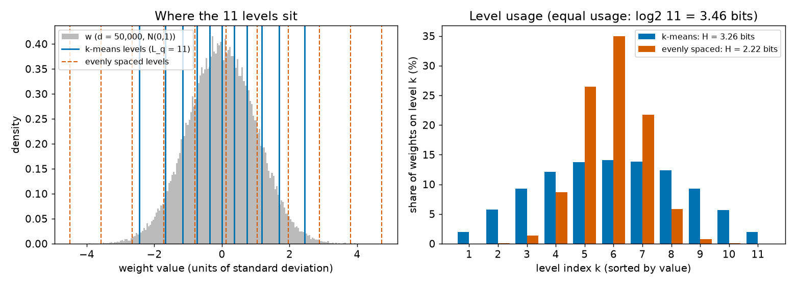
Left: histogram of the Gaussian w with the 11 k-means levels (solid) and 11 evenly spaced levels (dashed). Right: share of coordinates on each level.

At $L_q = 11$ and an ideal entropy code the whole vector costs 162,948 bits = 19.89 KB, 9.8 times less than float32. Arithmetic coding gets within 2 bits of this (Chapter 22).

Step 3 — learned levels versus an entropy-coded even grid¶

Does learning the levels give the smallest error for a given number of bits? Output [4] compares, at exactly the same entropy, the k-means codebook against an infinite evenly spaced grid (step chosen so that its usage entropy matches):

k-means $L_q$	$H$ (bits)	k-means MSE	grid step	grid MSE	grid levels used	grid / k-means MSE
5	2.1984	0.08099	0.9348	0.07280	11	0.899
11	3.2590	0.01941	0.4356	0.01597	21	0.822
17	3.8730	0.00869	0.2832	0.00666	31	0.766

At equal bits, the even grid has lower squared error. k-means aims at the best codebook for a fixed number of levels (the right goal for a fixed-length code). Once the indices are entropy-coded, many lightly used levels are cheap, and an even grid with more levels wins on squared error. This is a classical fact of quantization theory (SOURCE: Gish and Pierce 1968, "Asymptotically efficient quantizing"), which our numbers reproduce.

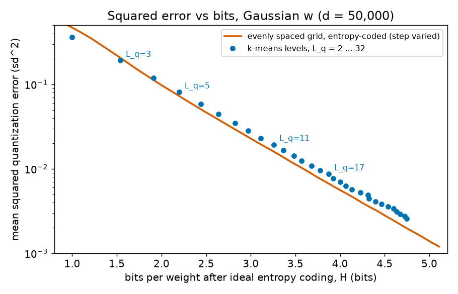
Mean squared error against bits per coordinate for k-means codebooks (dots, 2 to 32 levels) and an entropy-coded even grid (line).

Why does the paper learn a small codebook anyway? Our reading: QAT moves the levels to lower the training loss, which squared error only approximates; few levels keep the codebook and the table of level counts (which the decoder needs) small (erratum E18); and a fixed $L_q$ costs only one hyperparameter bit. The paper does not compare against an entropy-coded grid, so whether a grid would give a tighter bound is open.

Going deeper: the high-resolution formulas behind the grid numbers

MY EXPLANATION Let $f$ be the density of the coordinates (here the normal density with standard deviation $\sigma$) and let the grid step be $\text{step}$, small compared with $\sigma$.

Error. Inside one cell of width $\text{step}$, $f$ is nearly flat, so a coordinate's position in its cell is nearly uniform and the error $e$ is nearly uniform on $[-\text{step}/2, \text{step}/2]$. Its mean square is

\[ \frac{1}{\text{step}}\int_{-\text{step}/2}^{\text{step}/2} e^2\,de = \frac{1}{\text{step}}\cdot\frac{2}{3}\Big(\frac{\text{step}}{2}\Big)^3 = \frac{\text{step}^2}{12}. \]

Bits. Picture one coordinate drawn at random from the density $f$ (that draw is the only randomness here). The probability that it lands in cell $j$ around the point $x_j$ is $p_j \approx f(x_j)\,\text{step}$. Then

\[ \begin{aligned} H &= -\sum_j p_j \log_2 p_j \approx -\sum_j f(x_j)\,\text{step}\,\big[\log_2 f(x_j) + \log_2 \text{step}\big] \\ &\approx -\int f(x)\log_2 f(x)\,dx \;-\; \log_2 \text{step} \;=\; h(f) - \log_2 \text{step}, \end{aligned} \]

using $\sum_j f(x_j)\,\text{step} \approx \int f = 1$. The quantity $h(f) = -\int f\log_2 f$ is the differential entropy of $f$, in bits. For a normal density with mean 0, $-\log_2 f(x) = \frac{x^2}{2\sigma^2}\log_2 e + \frac12\log_2(2\pi\sigma^2)$; averaging with $\mathbb E[x^2] = \sigma^2$ gives

\[ h = \tfrac12\log_2 e + \tfrac12 \log_2(2\pi\sigma^2) = \tfrac12\log_2(2\pi e\,\sigma^2). \]

Check against output [4] (sample $\sigma = 1.0014$, so $h = 2.0491$ bits). For the 11-level match the step is 0.4356: $\text{step}^2/12 = 0.01581$ against the measured 0.01597, and $h - \log_2\text{step} = 2.0491 + 1.1989 = 3.2480$ bits against the measured 3.2590. For the coarser 5-level match (step 0.9348) the bits formula is off by about 0.05 bits (2.1463 against 2.1983), as expected when the step is no longer small.

Combining the two formulas: one extra bit per coordinate ($H$ up by 1) means $\log_2\text{step}$ down by 1, so the step halves and $\text{step}^2/12$ falls by a factor of 4. That is why the grid curve in the figure is close to a straight line on the log scale, falling by about a factor of 4 per bit. The k-means dots fall at a similar, slightly slower rate here; we do not derive their high-resolution formula.

Step 4 — gradients through the quantizer, by hand¶

Output [5] uses six coordinates, levels $c = (-1, 0, 1)$ and a quadratic loss. The coordinates $w = (+0.276, +0.657, +0.264, -1.043, +0.724, +0.357)$ round to $\hat w = (0, 1, 0, -1, 1, 0)$, and the loss is 8.5603.

True derivative of the loss with respect to each $w_i$ (finite differences): $+0.000$ for all six.
STE stand-in $\partial\mathcal L/\partial \hat w_i$: $+8.295, +4.680, -0.255, +0.629, +1.447, -0.114$.
Codebook gradient (cluster sums): level $-1$ gets $+0.62912$ (only coordinate 4); level $0$ gets $8.295 - 0.255 - 0.114 = 7.926$, printed as $+7.92535$; level $1$ gets $4.680 + 1.447 = 6.127$, printed as $+6.12764$. Finite differences agree to $1.0\times10^{-9}$.

Step 5 — QAT on a small network¶

Output [7]. A toy classifier: a network with 20 inputs, 32 hidden units and one output (a yes/no probability), $D = 705$ parameters, trained only through a random subspace, $\theta = \theta_0 + Qw$ with $d = 150$ and $Q$ a random matrix with orthonormal columns (playing the role of $P$). Labels come from a fixed random "teacher" network; there are 4,000 training and 20,000 test examples. Loss is the log-loss of Chapter 7 in nats per example.

(a) Full precision: 1,500 Adam steps give training loss 0.2073 and test loss 0.3121.
(b) Round after training: k-means levels on the trained $w$, no further training.
(c) QAT: start from (b) and run 400 Adam steps (step size 0.05, decayed along a cosine curve to 0) on $w$ and $c$, with the STE and the codebook gradient.

"Gap recovered" is $(\text{b} - \text{c})/(\text{b} - \text{a})$ on the training loss. "Levels changed" is the share of coordinates whose assigned level differs at the end of QAT.

$L_q$	(b) train	(b) test	(c) train	(c) test	gap recovered	levels changed	$H$ after QAT (bits)
3	0.4254	0.4647	0.2897	0.3026	62.2 %	28.7 %	1.578
5	0.3999	0.4470	0.2640	0.2917	70.6 %	43.3 %	2.264
11	0.2624	0.3433	0.2308	0.2899	57.3 %	56.7 %	3.441
17	0.2289	0.3314	0.2226	0.2965	29.5 %	61.3 %	3.989

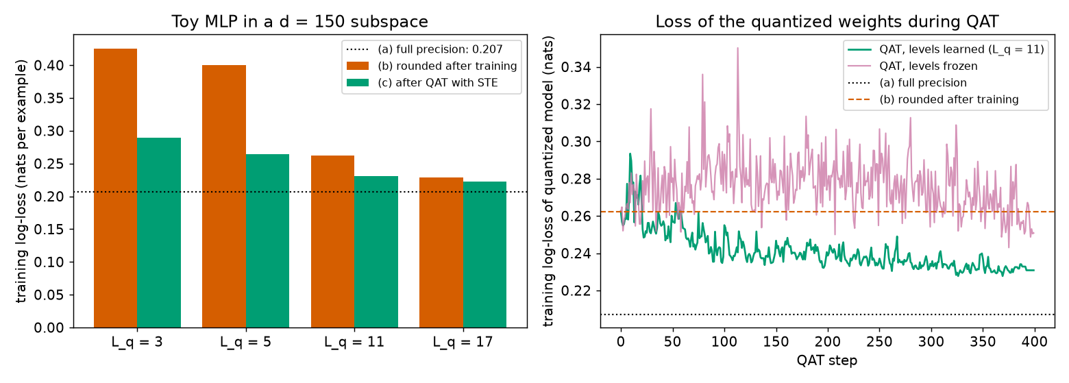
Left: training log-loss for full precision, rounding after training, and QAT. Right: loss of the quantized model during QAT at 11 levels, with levels learned or frozen.

What to notice:

Rounding alone hurts most with few levels (0.4254 at $L_q = 3$ against 0.2073). QAT recovers 57.3 % to 70.6 % of the gap at 3, 5 and 11 levels. At $L_q = 17$ it recovers only 29.5 %, but there was little to recover (0.2289 against 0.2073).
QAT really moves things: at $L_q = 11$, 56.7 % of coordinates end on a different level than they started.
Learning the levels matters. With the codebook frozen at its k-means start, QAT at 11 levels reaches only 0.2508 training loss (test 0.3196), against 0.2308 with learned levels, and its training curve is much noisier (right panel): with fixed levels, the STE makes coordinates hop back and forth across midpoints, as in the one-weight example above.
In this toy the QAT test losses are lower than the full-precision test loss 0.3121, because the full-precision model overfits (train 0.2073, test 0.3121). This is one toy with one seed; it suggests, but does not show, that quantization can act as a regularizer (anything that limits how closely a model can fit its training data, and so can reduce overfitting).
The trained $w$ here has sd 2.094 and its 11 k-means levels span $-4.23$ to $+3.75$; levels are always in the units of $w$, which is why they are learned from $w$ rather than fixed in advance.

Going deeper¶

Everything in this section is MY EXPLANATION unless tagged. The collapsible blocks of this chapter, in reading order:

Proof that Lloyd's algorithm never increases the squared error, and stops (with the 9-point local optimum).
The derivative of the nearest-level map is 0 almost everywhere.
The codebook gradient is exact.
The STE has no guarantee — a one-weight example.
The high-resolution formulas behind the grid numbers ($\text{step}^2/12$ and $h - \log_2 \text{step}$).

Going deeper: what exactly is stored, and what is thrown away

MY EXPLANATION After QAT the decoder receives: the codebook $c$ (e.g. 11 numbers at 16 bits), the level counts or probabilities needed by the arithmetic decoder, the arithmetic-coded index sequence $q(1),\dots,q(d)$, and the hyperparameter choices (including $L_q$). From these it rebuilds $\hat w$ exactly, then $\theta = \theta_0 + \mathrm{LoRA}(\phi_0 + P\hat w)$, that is, the SubLoRA map with $\hat w$ in place of $w$ (Chapter 20; $\theta_0$, $\phi_0$ and $P$ come from seeds). The full-precision $w$ is never stored. This matters for the bound: the hypothesis $\hat h$ whose risk is measured must be the quantized model, because that is the model whose description length is $C(h)$. PAPER App. C, Algorithm 1 line 5, p. 15 Algorithm 1 accordingly evaluates the empirical risk at $\hat w$, not $w$.

Common misconceptions¶

Everything in this section is MY EXPLANATION; numbers are from output [1]–[7].

Misconception: The paper quantizes all 124 million GPT-2 weights. — Actually: only the $d$ subspace coordinates ($d \le 200{,}000$, PAPER App. E, p. 16) are quantized; $\theta_0$, $\phi_0$ and $P$ come from seeds. Quantizing all $D = 123{,}689{,}472$ parameters at 4 bits would cost 494.8 million bits.
Misconception: With 11 levels each weight costs 4 bits. — Actually: 4 bits is the fixed-length price. Entropy coding costs at most $\log_2 11 = 3.4594$ bits, and less when usage is uneven: 3.2590 bits for k-means on Gaussian data, 2.709 bits per coordinate for the paper's best model (everything in its reported compressed size included).
Misconception: The straight-through estimator computes the gradient of the quantized network. — Actually: that gradient with respect to $w$ is zero almost everywhere. The STE substitutes the gradient with respect to $\hat w$; it is a useful pretence without a guarantee (in the one-weight example it averages loss 0.2400 where 0.1600 was available). The codebook gradient, by contrast, is exact.
Misconception: k-means finds the best codebook. — Actually: Lloyd's algorithm only reaches a fixed point; in the 9-point example it stops at squared error 154.5 while 6 is possible.
Misconception: Learned levels always beat evenly spaced ones. — Actually: for the same number of levels, usually yes (MSE 0.01941 against 0.07111 at 11 levels). For the same number of bits after entropy coding, an even grid has lower squared error (ratio 0.822 at 3.2590 bits).
Misconception: QAT makes the quantized model as good as the full-precision one. — Actually: it closes part of the gap; in our toy 57.3 % of the training-loss gap at 11 levels.

Self-test¶

Questions and answers are MY EXPLANATION; numbers are from output [1]–[3].

Q1. Using output [2] for $L_q = 11$ and $d = 50{,}000$: how many bits does $\hat w$'s index sequence cost with a fixed-length code, and with an ideal entropy code? How many times smaller is the second than float32?

Answer

Fixed length: $\lceil\log_2 11\rceil = 4$ bits per index, so $4 \times 50{,}000 = 200{,}000$ bits (24.414 KB). Ideal entropy code: $d \cdot H = 50{,}000 \times 3.2590 = 162{,}948$ bits (19.89 KB); arithmetic coding gets within 2 bits of this. Float32 is $32 \times 50{,}000 = 1{,}600{,}000$ bits, which is $32/3.2590 = 9.8$ times larger. The codebook (176 bits at 16 bits per level) and counts come on top. Units: bits throughout; KB means 8,192 bits.

Q2. Algorithm 1, line 12, updates $w$ by $w \leftarrow w - \rho\nabla_w\mathcal L(w,c)$, where the loss uses $\hat w$. Read literally, what happens? What does the straight-through estimator change, and is the update of $c$ also an approximation?

Answer

Literally, nothing happens to $w$: $\hat w$ is a staircase function of $w$, so $\nabla_w\mathcal L = 0$ almost everywhere (erratum E17). The STE replaces $\partial\hat w_i/\partial w_j$ by $\mathbf 1[i=j]$, so $w$ is moved by $-\rho\,\partial\mathcal L/\partial\hat w$, the gradient evaluated at the quantized weights; $w$ drifts until it crosses a midpoint and $\hat w_i$ changes level. The update of $c$ is not an approximation: away from midpoints the assignments do not change under small moves of $c$, so $\partial\mathcal L/\partial c_k = \sum_{i:\,q(i)=k}\partial\mathcal L/\partial\hat w_i$ exactly.

Q3. For the points $0,1,2,10,11,12,20,21,22$ and three levels, show that $(0, 1.5, 16)$ is a fixed point of Lloyd's algorithm and compute its squared error. Is it the best codebook?

Answer

Midpoints: $(0+1.5)/2 = 0.75$ and $(1.5+16)/2 = 8.75$. So $0$ goes to level 0, $1$ and $2$ to level 1.5, and the six points from 10 to 22 to level 16. The cluster means are $0$, $1.5$ and $(10+11+12+20+21+22)/6 = 96/6 = 16$: unchanged, so it is a fixed point. Squared error: $0 + (0.5^2 + 0.5^2) + (6^2+5^2+4^2+4^2+5^2+6^2) = 0.5 + 154 = 154.5$. It is not the best: levels $(1, 11, 21)$ give $3 \times 2 = 6$ (each group of three has squared error $1 + 0 + 1 = 2$). Lloyd's algorithm reaches a local optimum, not necessarily the global one (output [3]).

Code for this chapter¶

Run it from the project root:

.venv/Scripts/python explainer/code/ch21_quantize.py

Source: ch21_quantize.py

"""Chapter 21 demo: quantization, k-means (Lloyd's algorithm) and quantization-aware training (QAT).

What this script reproduces or illustrates (every number quoted in Chapter 21 comes from here):
  [1] Bit arithmetic: ceil(log2 L_q) bits per weight for a fixed-length code (4 for 11 levels, 5 for 17),
      the entropy ceiling log2 L_q, float32 storage of d = 50,000 coordinates, the paper's best model
      (Fig. 2 left, compressed size read exactly from the PDF by fig_extract.py -> bits per coordinate),
      and why only the d subspace coordinates (not GPT-2's D parameters) are quantized.
  [2] Lloyd's algorithm (1-D k-means) on a Gaussian vector w (d = 50,000, seed 0) for L_q in {3, 5, 11, 17}:
      squared error never increases (asserted), mean squared quantization error, usage entropy (bits/weight),
      total d*H bits vs float32; comparison with evenly spaced ("uniform") levels.
  [3] Lloyd's algorithm can stop at a bad local optimum (9-point example).
  [4] Learned levels vs an entropy-coded uniform grid: squared error at equal bits/weight.
  [5] Gradients through the nearest-level assignment: the true derivative wrt w is 0; the
      straight-through estimator (STE) replaces it; the codebook gradient sum_{i: q(i)=k} dL/dw_hat_i
      equals a finite difference (it is an exact derivative almost everywhere).
  [6] STE has no guarantee: a 1-D example where STE with a fixed codebook keeps flipping between two levels.
  [7] QAT on a toy: a small MLP trained in a random subspace of dimension d = 150; training log-loss of
      (a) full-precision w, (b) w rounded to k-means levels after training, (c) after 400 steps of QAT
      with STE (learning w and the levels together).
Figures: docs/assets/fig/ch21_levels.png, ch21_rate_distortion.png, ch21_qat.png
Output:  code/outputs/ch21_quantize.txt
Deterministic (numpy default_rng seeds 0, 1, 2). CPU only; runtime about 20-40 s.
"""
from __future__ import annotations

import json
import math
import os
import sys
from pathlib import Path

for _v in ("OPENBLAS_NUM_THREADS", "OMP_NUM_THREADS", "MKL_NUM_THREADS"):
    os.environ.setdefault(_v, "1")  # small matrices: one BLAS thread is faster and fully deterministic

import numpy as np  # noqa: E402
import matplotlib

matplotlib.use("Agg")
import matplotlib.pyplot as plt  # noqa: E402

HERE = Path(__file__).resolve().parent
sys.path.insert(0, str(HERE))
import pacbound as pb  # noqa: E402

OUT_TXT = HERE / "outputs" / "ch21_quantize.txt"
FIG_DIR = HERE.parent / "docs" / "assets" / "fig"
FIG_JSON = HERE / "outputs" / "fig_extract.json"
OUT_TXT.parent.mkdir(parents=True, exist_ok=True)
FIG_DIR.mkdir(parents=True, exist_ok=True)

BLUE, VERM, GREEN, PINK, ORANGE, SKY = "#0072B2", "#D55E00", "#009E73", "#CC79A7", "#E69F00", "#56B4E9"
LINES: list[str] = []


def say(s: str = "") -> None:
    print(s)
    LINES.append(s)


# ---------------------------------------------------------------------------
# Helpers
# ---------------------------------------------------------------------------
def entropy_bits(counts) -> float:
    """Empirical entropy -sum p log2 p (bits per symbol) of a vector of counts."""
    p = np.asarray(counts, dtype=float)
    p = p[p > 0] / p.sum()
    return float(-(p * np.log2(p)).sum())


def nearest(x: np.ndarray, c: np.ndarray) -> np.ndarray:
    """Nearest-level assignment q(i) = argmin_k |x_i - c_k| (ties -> lowest index)."""
    return np.argmin(np.abs(x[:, None] - c[None, :]), axis=1)


def lloyd_1d(x: np.ndarray, c0: np.ndarray, max_iter: int = 20000):
    """Lloyd's algorithm in 1-D. x must be sorted. Returns (levels, counts, sse_history, iterations).
    sse_history interleaves the squared error after each assignment step and after each update step."""
    x = np.asarray(x, float)
    s1 = np.concatenate([[0.0], np.cumsum(x)])
    s2 = np.concatenate([[0.0], np.cumsum(x * x)])
    c = np.sort(np.asarray(c0, float))
    hist, prev = [], None
    for it in range(1, max_iter + 1):
        # assignment step: in 1-D the nearest-level cells are intervals cut at midpoints
        cuts = np.searchsorted(x, (c[:-1] + c[1:]) / 2.0)
        edges = np.concatenate([[0], cuts, [len(x)]])
        n = np.diff(edges).astype(float)
        sm = s1[edges[1:]] - s1[edges[:-1]]
        sq = s2[edges[1:]] - s2[edges[:-1]]
        hist.append(float((sq - 2 * c * sm + n * c * c).sum()))
        if prev is not None and np.array_equal(cuts, prev):
            return c, n.astype(int), hist, it
        prev = cuts
        # update step: each level moves to the mean of its cell (empty cells keep their level)
        c = np.where(n > 0, sm / np.maximum(n, 1), c)
        hist.append(float((sq - 2 * c * sm + n * c * c).sum()))
    return c, n.astype(int), hist, max_iter


def lloyd_small(x: np.ndarray, c: np.ndarray, iters: int = 200) -> np.ndarray:
    """Plain Lloyd's algorithm for small unsorted vectors (used in the toy)."""
    c = np.asarray(c, float).copy()
    for _ in range(iters):
        a = nearest(x, c)
        c = np.array([x[a == k].mean() if np.any(a == k) else c[k] for k in range(len(c))])
    return c


def main() -> None:
    # =======================================================================
    say("[1] Bits per weight (fixed-length code vs entropy ceiling vs float32)")
    for L in pb.QLEVEL_GRID:
        say(f"  L_q = {L}: fixed length ceil(log2 L_q) = {math.ceil(math.log2(L))} bits;"
            f" entropy ceiling log2 L_q = {math.log2(L):.4f} bits")
    d = 50_000
    say(f"  d = {d:,} coordinates: float32 {32 * d:,} bits = {32 * d / 8192:.2f} KB (1 KB = 8192 bits);"
        f" 4 bits each {4 * d:,} bits = {4 * d / 8192:.3f} KB; 5 bits each {5 * d:,} bits")
    f2 = json.loads(FIG_JSON.read_text(encoding="utf-8"))["figure2"]["left"]["compressed_size_kb"]
    best_kb = [pt["value"] for pt in f2 if abs(pt["d"] - 50_000) < 250][0]
    best_bits = best_kb * 8192
    say(f"  [PAPER Fig. 2 left, fig_extract.py] best model d = 50,000: {best_kb:.4f} KB = {best_bits:,.0f} bits"
        f" = {best_bits / d:.3f} bits/coordinate; float32 is {32 * d / best_bits:.1f}x larger")
    D = pb.gpt2_params(12, 768)
    say(f"  GPT-2 small (nanoGPT count) D = {D:,} parameters = {D / d:,.0f} x d;"
        f" quantizing all D at 4 bits = {4 * D / 1e6:,.1f} Mbit, at {best_bits / d:.3f} bits = {D * best_bits / d / 1e6:,.1f} Mbit")
    say(f"  choosing L_q from {{11, 17}} costs log2 2 = {math.log2(2):.0f} bit in the prior")
    say("  codebook: " + "; ".join(f"L_q = {L}: 16 bits each {16 * L} bits, 32 bits each {32 * L} bits"
                                    for L in pb.QLEVEL_GRID))

    # =======================================================================
    say("[2] Lloyd's algorithm (1-D k-means) on w ~ N(0,1), d = 50,000 (seed 0); MSE in units of sd^2")
    rng = np.random.default_rng(0)
    w = np.sort(rng.standard_normal(d))
    say(f"  sample: mean {w.mean():+.4f}, sd {w.std():.4f}, min {w.min():.3f}, max {w.max():.3f}")
    say("  L_q | iters | k-means MSE  max|err|  H bits  d*H bits  KB    f32/(dH) | uniform MSE  H bits")
    results = {}
    for L in [3, 5, 11, 17]:
        c0 = np.quantile(w, (np.arange(L) + 0.5) / L)
        c, n, hist, its = lloyd_1d(w, c0)
        assert all(b <= a + 1e-9 * max(1.0, a) for a, b in zip(hist, hist[1:])), "SSE increased!"
        a = nearest(w, c)
        err = w - c[a]
        mse, H = float(np.mean(err ** 2)), entropy_bits(n)
        cu = np.linspace(w.min(), w.max(), L)
        au = nearest(w, cu)
        mse_u, H_u = float(np.mean((w - cu[au]) ** 2)), entropy_bits(np.bincount(au, minlength=L))
        results[L] = dict(c=c, n=n, mse=mse, H=H, cu=cu, nu=np.bincount(au, minlength=L), mse_u=mse_u, H_u=H_u,
                          hist=hist)
        say(f"  {L:>3} | {its:>5} | {mse:.5f}     {np.abs(err).max():.3f}    {H:.4f}  {d * H:>9,.0f} {d * H / 8192:6.2f}   {32 / H:5.1f}x"
            f"   | {mse_u:.5f}      {H_u:.4f}")
    say(f"  squared error never increased in any run (asserted); L_q=11 SSE: start {results[11]['hist'][0]:,.1f}"
        f" -> end {results[11]['hist'][-1]:,.1f}")
    r = results[11]
    say("  L_q = 11 k-means levels: " + " ".join(f"{v:+.3f}" for v in r["c"]))
    say("  usage %:                 " + " ".join(f"{100 * v / d:6.2f}" for v in r["n"]))
    say("  L_q = 11 uniform levels: " + " ".join(f"{v:+.3f}" for v in r["cu"]))
    say("  usage %:                 " + " ".join(f"{100 * v / d:6.2f}" for v in r["nu"]))
    say(f"  total at d*H: 11 levels {d * r['H']:,.0f} bits = {d * r['H'] / 8192:.2f} KB vs float32 {32 * d:,} bits"
        f" ({32 / r['H']:.1f}x smaller)")

    # =======================================================================
    say("[3] Lloyd's algorithm can stop at a bad local optimum (points 0,1,2,10,11,12,20,21,22; L_q = 3)")
    xs = np.array([0, 1, 2, 10, 11, 12, 20, 21, 22], float)
    for name, init in [("start (0, 1, 16)", [0, 1, 16]), ("start (1, 11, 21)", [1, 11, 21])]:
        c, n, hist, its = lloyd_1d(xs, np.array(init, float))
        say(f"  {name}: final levels ({', '.join(f'{v:g}' for v in c)}), counts {[int(v) for v in n]},"
            f" squared error {hist[-1]:g}")

    # =======================================================================
    say("[4] Learned (k-means) levels vs an entropy-coded uniform grid, same w (MSE at equal bits/weight)")

    def unif_grid(step):
        q = np.round(w / step)
        _, cnt = np.unique(q, return_counts=True)
        return float(np.mean((w - step * q) ** 2)), entropy_bits(cnt), len(cnt)

    for L in [5, 11, 17]:
        target = results[L]["H"]
        lo, hi = 1e-3, 5.0
        for _ in range(60):  # entropy falls as the step grows: bisect on the step
            mid = math.sqrt(lo * hi)
            if unif_grid(mid)[1] > target:
                lo = mid
            else:
                hi = mid
        mse_g, H_g, used = unif_grid(math.sqrt(lo * hi))
        say(f"  k-means L_q={L:>2}: H = {target:.4f} bits, MSE {results[L]['mse']:.5f} | grid step"
            f" {math.sqrt(lo * hi):.4f}: H = {H_g:.4f} bits, MSE {mse_g:.5f} ({used} levels used);"
            f" grid/k-means MSE = {mse_g / results[L]['mse']:.3f}")
        step = math.sqrt(lo * hi)
        h_diff = 0.5 * math.log2(2 * math.pi * math.e * float(np.var(w)))
        say(f"      high-resolution check: step^2/12 = {step ** 2 / 12:.5f} (MSE {mse_g:.5f});"
            f" h(N(0,sd^2)) - log2 step = {h_diff:.4f} + {-math.log2(step):.4f} = {h_diff - math.log2(step):.4f} bits"
            f" (H {H_g:.4f})")
    km_curve = []
    for L in range(2, 33):
        c, n, _, _ = lloyd_1d(w, np.quantile(w, (np.arange(L) + 0.5) / L))
        km_curve.append((entropy_bits(n), float(np.mean((w - c[nearest(w, c)]) ** 2)), L))
    grid_curve = [unif_grid(s)[:2] for s in np.geomspace(0.12, 4.0, 60)]

    # =======================================================================
    say("[5] Gradients through w_hat_i = c_q(i): true derivative, STE, codebook gradient (seed 1)")
    rng1 = np.random.default_rng(1)
    dd, cc = 6, np.array([-1.0, 0.0, 1.0])
    wv = rng1.normal(0, 0.8, dd)
    A = rng1.standard_normal((4, dd))
    bvec = rng1.standard_normal(4)

    def loss_of(wvec, cvec):
        wh = cvec[nearest(wvec, cvec)]
        return 0.5 * float(np.sum((A @ wh - bvec) ** 2))

    q = nearest(wv, cc)
    wh = cc[q]
    g_hat = A.T @ (A @ wh - bvec)  # dL/dw_hat
    eps = 1e-6
    fd_w = np.array([(loss_of(wv + eps * e, cc) - loss_of(wv - eps * e, cc)) / (2 * eps) for e in np.eye(dd)])
    fd_c = np.array([(loss_of(wv, cc + eps * e) - loss_of(wv, cc - eps * e)) / (2 * eps) for e in np.eye(3)])
    g_c = np.bincount(q, weights=g_hat, minlength=3)
    say("  w      = " + " ".join(f"{v:+.3f}" for v in wv) + "   levels c = (" + ", ".join(f"{v:g}" for v in cc) + ")")
    say("  w_hat  = " + " ".join(f"{v:+.3f}" for v in wh) + f"   loss = {loss_of(wv, cc):.4f}")
    say("  finite-difference dL/dw (true derivative): " + " ".join(f"{v:+.3f}" for v in fd_w))
    say("  STE dL/dw := dL/dw_hat                   : " + " ".join(f"{v:+.3f}" for v in g_hat))
    say("  codebook: sum_{i:q(i)=k} dL/dw_hat_i     : " + " ".join(f"{v:+.5f}" for v in g_c))
    say("  codebook: finite difference dL/dc_k      : " + " ".join(f"{v:+.5f}" for v in fd_c)
        + f"   max |diff| = {np.abs(g_c - fd_c).max():.1e}")
    assert np.abs(fd_w).max() == 0.0 and np.abs(g_c - fd_c).max() < 1e-6

    # =======================================================================
    say("[6] STE has no guarantee: L(w_hat) = (w_hat - 0.4)^2, levels {0, 1}, SGD lr 0.05, start w = 0.2")
    for learn_c in [False, True]:
        wl, c = 0.2, np.array([0.0, 1.0])
        at_one, losses = 0, []
        for t in range(200):
            k = int(np.argmin(np.abs(wl - c)))
            g = 2 * (c[k] - 0.4)
            losses.append((c[k] - 0.4) ** 2)
            at_one += (k == 1)
            wl -= 0.05 * g
            if learn_c:
                c[k] -= 0.05 * g
        tag = "levels learned too" if learn_c else "levels fixed     "
        say(f"  {tag}: steps on level 1 = {at_one}/200; mean loss last 100 = {np.mean(losses[100:]):.4f};"
            f" final w = {wl:.3f}, levels = ({c[0]:.3f}, {c[1]:.3f})")
    say("  best fixed-level choice: w_hat = 0, loss 0.1600")

    # =======================================================================
    say("[7] QAT toy: MLP 20-32-1 (D = 705) trained as theta = theta0 + Q w, d = 150; log-loss in nats/example")
    rng2 = np.random.default_rng(2)
    Din, Hh, dsub, m, mt = 20, 32, 150, 4000, 20000
    X, Xt = rng2.standard_normal((m, Din)), rng2.standard_normal((mt, Din))
    W1, v1 = rng2.standard_normal((Din, 16)) / np.sqrt(Din), 2 * rng2.standard_normal(16)
    sig = lambda z: 1 / (1 + np.exp(-z))  # noqa: E731
    teacher = lambda Z: np.tanh(2 * Z @ W1) @ v1  # noqa: E731
    y = (rng2.random(m) < sig(teacher(X))).astype(float)
    yt = (rng2.random(mt) < sig(teacher(Xt))).astype(float)
    Dm = Din * Hh + 2 * Hh + 1
    theta0 = 0.1 * rng2.standard_normal(Dm)
    Q, _ = np.linalg.qr(rng2.standard_normal((Dm, dsub)))

    def loss_grad(wvec, XX, yy, grad=True):
        th = theta0 + Q @ wvec
        Aw, bw, vw, c0 = th[:Din * Hh].reshape(Din, Hh), th[Din * Hh:Din * Hh + Hh], th[Din * Hh + Hh:-1], th[-1]
        h = np.tanh(XX @ Aw + bw)
        z = h @ vw + c0
        l = float(np.mean(np.logaddexp(0, z) - yy * z))
        if not grad:
            return l
        dz = (sig(z) - yy) / len(yy)
        dpre = np.outer(dz, vw) * (1 - h ** 2)
        gth = np.concatenate([(XX.T @ dpre).ravel(), dpre.sum(0), h.T @ dz, [dz.sum()]])
        return l, Q.T @ gth

    class Adam:
        def __init__(self, n, lr):
            self.m, self.v, self.t, self.lr = np.zeros(n), np.zeros(n), 0, lr

        def step(self, g, f=1.0):
            self.t += 1
            self.m = 0.9 * self.m + 0.1 * g
            self.v = 0.999 * self.v + 0.001 * g * g
            mh, vh = self.m / (1 - 0.9 ** self.t), self.v / (1 - 0.999 ** self.t)
            return f * self.lr * mh / (np.sqrt(vh) + 1e-8)

    wfp, opt = np.zeros(dsub), Adam(dsub, 0.02)
    for _ in range(1500):
        _, g = loss_grad(wfp, X, y)
        wfp -= opt.step(g)
    fp_tr, fp_te = loss_grad(wfp, X, y, False), loss_grad(wfp, Xt, yt, False)
    say(f"  (a) full precision after 1,500 Adam steps: train {fp_tr:.4f}, test {fp_te:.4f}"
        f" (|grad| = {np.linalg.norm(loss_grad(wfp, X, y)[1]):.1e}; w sd {wfp.std():.3f})")
    say(f"  m = {m:,} train / {mt:,} test examples; QAT: 400 Adam steps, lr 0.05 with cosine decay, k-means start")
    say("  L_q | (b) round after training | (c) after QAT          | gap recovered | levels changed | H bits")
    say("      |   train     test         |   train     test       |               |                |")
    qat_rows, curve11 = {}, None

    def qat(L, learn_c=True, steps=400, lr=0.05):
        c = lloyd_small(wfp, np.quantile(wfp, (np.arange(L) + 0.5) / L))
        a0 = nearest(wfp, c)
        wq, cq = wfp.copy(), c.copy()
        ow, oc, curve = Adam(dsub, lr), Adam(L, lr), []
        for t in range(steps):
            f = 0.5 * (1 + math.cos(math.pi * t / steps))
            a = nearest(wq, cq)
            l, g = loss_grad(cq[a], X, y)       # forward pass with the QUANTIZED weights
            curve.append(l)
            wq -= ow.step(g, f)                 # STE: dL/dw_i := dL/dw_hat_i
            if learn_c:
                cq -= oc.step(np.bincount(a, weights=g, minlength=L), f)  # dL/dc_k = sum_{q(i)=k} dL/dw_hat_i
        a = nearest(wq, cq)
        return c, a0, cq, a, curve

    for L in [3, 5, 11, 17]:
        c, a0, cq, a, curve = qat(L)
        ptq_tr, ptq_te = loss_grad(c[a0], X, y, False), loss_grad(c[a0], Xt, yt, False)
        q_tr, q_te = loss_grad(cq[a], X, y, False), loss_grad(cq[a], Xt, yt, False)
        rec = (ptq_tr - q_tr) / (ptq_tr - fp_tr)
        qat_rows[L] = (ptq_tr, ptq_te, q_tr, q_te, rec)
        if L == 11:
            curve11 = curve
        say(f"  {L:>3} |   {ptq_tr:.4f}    {ptq_te:.4f}       |   {q_tr:.4f}    {q_te:.4f}     |"
            f"     {100 * rec:5.1f} %   |  {np.mean(a != a0) * 100:5.1f} %       |"
            f" {entropy_bits(np.bincount(a, minlength=L)):.3f}")
    c, a0, cq, a, curve_fix = qat(11, learn_c=False)
    say(f"  L_q = 11 with the codebook frozen at its k-means start: train {loss_grad(cq[a], X, y, False):.4f},"
        f" test {loss_grad(cq[a], Xt, yt, False):.4f}")
    say(f"  L_q = 11 levels before QAT: " + " ".join(f"{v:+.2f}" for v in lloyd_small(
        wfp, np.quantile(wfp, (np.arange(11) + 0.5) / 11))))

    # =======================================================================
    # Figures
    plt.rcParams.update({"font.size": 11})
    r = results[11]
    fig, ax = plt.subplots(1, 2, figsize=(12, 4.3))
    ax[0].hist(w, bins=200, density=True, color="#BBBBBB", label="w (d = 50,000, N(0,1))")
    for i, v in enumerate(r["c"]):
        ax[0].axvline(v, color=BLUE, lw=1.6, label="k-means levels (L_q = 11)" if i == 0 else None)
    for i, v in enumerate(r["cu"]):
        ax[0].axvline(v, color=VERM, lw=1.2, ls="--", label="evenly spaced levels" if i == 0 else None)
    ax[0].set_xlabel("weight value (units of standard deviation)")
    ax[0].set_ylabel("density")
    ax[0].set_title("Where the 11 levels sit")
    ax[0].legend(fontsize=9, loc="upper left")
    idx = np.arange(11)
    ax[1].bar(idx - 0.2, 100 * r["n"] / d, 0.4, color=BLUE, label=f"k-means: H = {r['H']:.2f} bits")
    ax[1].bar(idx + 0.2, 100 * r["nu"] / d, 0.4, color=VERM, label=f"evenly spaced: H = {r['H_u']:.2f} bits")
    ax[1].set_xticks(idx, [str(i + 1) for i in idx])
    ax[1].set_xlabel("level index k (sorted by value)")
    ax[1].set_ylabel("share of weights on level k (%)")
    ax[1].set_title(f"Level usage (equal usage: log2 11 = {math.log2(11):.2f} bits)")
    ax[1].legend(fontsize=9)
    fig.tight_layout()
    fig.savefig(FIG_DIR / "ch21_levels.png", dpi=130)
    plt.close(fig)

    fig, ax = plt.subplots(figsize=(7, 4.5))
    gy, gx = zip(*grid_curve)  # unif_grid returns (mse, H)
    ax.semilogy(gx, gy, color=VERM, lw=2, label="evenly spaced grid, entropy-coded (step varied)")
    kx, ky, kl = zip(*km_curve)
    ax.semilogy(kx, ky, "o", color=BLUE, ms=5, label="k-means levels, L_q = 2 ... 32")
    for x0, y0, L in km_curve:
        if L in (3, 5, 11, 17):
            ax.annotate(f"L_q={L}", (x0, y0), textcoords="offset points", xytext=(6, 4), fontsize=9, color=BLUE)
    ax.set_xlabel("bits per weight after ideal entropy coding, H (bits)")
    ax.set_ylabel("mean squared quantization error (sd^2)")
    ax.set_xlim(0.8, 5.2)
    ax.set_ylim(1e-3, 0.5)
    ax.set_title("Squared error vs bits, Gaussian w (d = 50,000)")
    ax.legend(fontsize=9)
    fig.tight_layout()
    fig.savefig(FIG_DIR / "ch21_rate_distortion.png", dpi=130)
    plt.close(fig)

    fig, ax = plt.subplots(1, 2, figsize=(12, 4.3))
    Ls = [3, 5, 11, 17]
    xi = np.arange(len(Ls))
    ax[0].axhline(fp_tr, color="k", lw=1.2, ls=":", label=f"(a) full precision: {fp_tr:.3f}")
    ax[0].bar(xi - 0.2, [qat_rows[L][0] for L in Ls], 0.4, color=VERM, label="(b) rounded after training")
    ax[0].bar(xi + 0.2, [qat_rows[L][2] for L in Ls], 0.4, color=GREEN, label="(c) after QAT with STE")
    ax[0].set_xticks(xi, [f"L_q = {L}" for L in Ls])
    ax[0].set_ylabel("training log-loss (nats per example)")
    ax[0].set_title("Toy MLP in a d = 150 subspace")
    ax[0].legend(fontsize=9)
    ax[1].plot(curve11, color=GREEN, lw=1.5, label="QAT, levels learned (L_q = 11)")
    ax[1].plot(curve_fix, color=PINK, lw=1.2, alpha=0.8, label="QAT, levels frozen")
    ax[1].axhline(fp_tr, color="k", lw=1.2, ls=":", label="(a) full precision")
    ax[1].axhline(qat_rows[11][0], color=VERM, lw=1.2, ls="--", label="(b) rounded after training")
    ax[1].set_xlabel("QAT step")
    ax[1].set_ylabel("training log-loss of quantized model (nats)")
    ax[1].set_title("Loss of the quantized weights during QAT")
    ax[1].legend(fontsize=9)
    fig.tight_layout()
    fig.savefig(FIG_DIR / "ch21_qat.png", dpi=130)
    plt.close(fig)

    OUT_TXT.write_text("\n".join(LINES) + "\n", encoding="utf-8")


if __name__ == "__main__":
    main()

Output:

[1] Bits per weight (fixed-length code vs entropy ceiling vs float32)
  L_q = 11: fixed length ceil(log2 L_q) = 4 bits; entropy ceiling log2 L_q = 3.4594 bits
  L_q = 17: fixed length ceil(log2 L_q) = 5 bits; entropy ceiling log2 L_q = 4.0875 bits
  d = 50,000 coordinates: float32 1,600,000 bits = 195.31 KB (1 KB = 8192 bits); 4 bits each 200,000 bits = 24.414 KB; 5 bits each 250,000 bits
  [PAPER Fig. 2 left, fig_extract.py] best model d = 50,000: 16.5325 KB = 135,434 bits = 2.709 bits/coordinate; float32 is 11.8x larger
  GPT-2 small (nanoGPT count) D = 123,689,472 parameters = 2,474 x d; quantizing all D at 4 bits = 494.8 Mbit, at 2.709 bits = 335.0 Mbit
  choosing L_q from {11, 17} costs log2 2 = 1 bit in the prior
  codebook: L_q = 11: 16 bits each 176 bits, 32 bits each 352 bits; L_q = 17: 16 bits each 272 bits, 32 bits each 544 bits
[2] Lloyd's algorithm (1-D k-means) on w ~ N(0,1), d = 50,000 (seed 0); MSE in units of sd^2
  sample: mean +0.0008, sd 1.0014, min -4.494, max 4.732
  L_q | iters | k-means MSE  max|err|  H bits  d*H bits  KB    f32/(dH) | uniform MSE  H bits
    3 |    24 | 0.19215     3.521    1.5393     76,964   9.39    20.8x   | 0.94292      0.1795
    5 |    24 | 0.08099     3.014    2.1984    109,918  13.42    14.6x   | 0.43429      1.0664
   11 |    73 | 0.01941     2.293    3.2590    162,948  19.89     9.8x   | 0.07111      2.2158
   17 |   277 | 0.00869     2.007    3.8730    193,650  23.64     8.3x   | 0.02763      2.8617
  squared error never increased in any run (asserted); L_q=11 SSE: start 1,955.2 -> end 970.7
  L_q = 11 k-means levels: -2.438 -1.680 -1.164 -0.744 -0.365 -0.004 +0.361 +0.746 +1.173 +1.687 +2.439
  usage %:                   2.02   5.71   9.25  12.09  13.72  14.08  13.84  12.39   9.30   5.65   1.95
  L_q = 11 uniform levels: -4.494 -3.572 -2.649 -1.726 -0.804 +0.119 +1.042 +1.964 +2.887 +3.809 +4.732
  usage %:                   0.00   0.10   1.41   8.65  26.45  34.99  21.78   5.82   0.74   0.05   0.00
  total at d*H: 11 levels 162,948 bits = 19.89 KB vs float32 1,600,000 bits (9.8x smaller)
[3] Lloyd's algorithm can stop at a bad local optimum (points 0,1,2,10,11,12,20,21,22; L_q = 3)
  start (0, 1, 16): final levels (0, 1.5, 16), counts [1, 2, 6], squared error 154.5
  start (1, 11, 21): final levels (1, 11, 21), counts [3, 3, 3], squared error 6
[4] Learned (k-means) levels vs an entropy-coded uniform grid, same w (MSE at equal bits/weight)
  k-means L_q= 5: H = 2.1984 bits, MSE 0.08099 | grid step 0.9348: H = 2.1983 bits, MSE 0.07280 (11 levels used); grid/k-means MSE = 0.899
      high-resolution check: step^2/12 = 0.07283 (MSE 0.07280); h(N(0,sd^2)) - log2 step = 2.0491 + 0.0972 = 2.1463 bits (H 2.1983)
  k-means L_q=11: H = 3.2590 bits, MSE 0.01941 | grid step 0.4356: H = 3.2590 bits, MSE 0.01597 (21 levels used); grid/k-means MSE = 0.822
      high-resolution check: step^2/12 = 0.01581 (MSE 0.01597); h(N(0,sd^2)) - log2 step = 2.0491 + 1.1989 = 3.2480 bits (H 3.2590)
  k-means L_q=17: H = 3.8730 bits, MSE 0.00869 | grid step 0.2832: H = 3.8730 bits, MSE 0.00666 (31 levels used); grid/k-means MSE = 0.766
      high-resolution check: step^2/12 = 0.00668 (MSE 0.00666); h(N(0,sd^2)) - log2 step = 2.0491 + 1.8200 = 3.8692 bits (H 3.8730)
[5] Gradients through w_hat_i = c_q(i): true derivative, STE, codebook gradient (seed 1)
  w      = +0.276 +0.657 +0.264 -1.043 +0.724 +0.357   levels c = (-1, 0, 1)
  w_hat  = +0.000 +1.000 +0.000 -1.000 +1.000 +0.000   loss = 8.5603
  finite-difference dL/dw (true derivative): +0.000 +0.000 +0.000 +0.000 +0.000 +0.000
  STE dL/dw := dL/dw_hat                   : +8.295 +4.680 -0.255 +0.629 +1.447 -0.114
  codebook: sum_{i:q(i)=k} dL/dw_hat_i     : +0.62912 +7.92535 +6.12764
  codebook: finite difference dL/dc_k      : +0.62912 +7.92535 +6.12764   max |diff| = 1.0e-09
[6] STE has no guarantee: L(w_hat) = (w_hat - 0.4)^2, levels {0, 1}, SGD lr 0.05, start w = 0.2
  levels fixed     : steps on level 1 = 77/200; mean loss last 100 = 0.2400; final w = 0.500, levels = (0.000, 1.000)
  levels learned too: steps on level 1 = 0/200; mean loss last 100 = 0.0000; final w = 0.600, levels = (0.400, 1.000)
  best fixed-level choice: w_hat = 0, loss 0.1600
[7] QAT toy: MLP 20-32-1 (D = 705) trained as theta = theta0 + Q w, d = 150; log-loss in nats/example
  (a) full precision after 1,500 Adam steps: train 0.2073, test 0.3121 (|grad| = 1.6e-04; w sd 2.094)
  m = 4,000 train / 20,000 test examples; QAT: 400 Adam steps, lr 0.05 with cosine decay, k-means start
  L_q | (b) round after training | (c) after QAT          | gap recovered | levels changed | H bits
      |   train     test         |   train     test       |               |                |
    3 |   0.4254    0.4647       |   0.2897    0.3026     |      62.2 %   |   28.7 %       | 1.578
    5 |   0.3999    0.4470       |   0.2640    0.2917     |      70.6 %   |   43.3 %       | 2.264
   11 |   0.2624    0.3433       |   0.2308    0.2899     |      57.3 %   |   56.7 %       | 3.441
   17 |   0.2289    0.3314       |   0.2226    0.2965     |      29.5 %   |   61.3 %       | 3.989
  L_q = 11 with the codebook frozen at its k-means start: train 0.2508, test 0.3196
  L_q = 11 levels before QAT: -4.23 -2.50 -1.68 -1.22 -0.58 -0.15 +0.48 +1.25 +1.86 +2.76 +3.75

Code	Bits per coordinate	Total for \(d = 50{,}000\)
float32	32	1,600,000 bits = 195.31 KB
fixed length, \(L_q = 11\)	\(\lceil\log_2 11\rceil = 4\)	200,000 bits = 24.414 KB
fixed length, \(L_q = 17\)	\(\lceil\log_2 17\rceil = 5\)	250,000 bits
entropy ceiling, \(L_q = 11\)	\(\log_2 11 = 3.4594\)	(at most)
entropy ceiling, \(L_q = 17\)	\(\log_2 17 = 4.0875\)	(at most)
paper's best model (Fig. 2 left)	2.709	135,434 bits = 16.5325 KB