11. Priors over hypotheses: Theorem A.1 and Eq. (1)¶
Where this fits
Prerequisites: Chapter 1 (probability, fixed versus random, "with probability at least \(1-\delta\)", failure probability), Chapter 2 (hypothesis, hypothesis space, empirical and expected risk, generalization bound, vacuous, deterministic versus stochastic predictor), Chapter 3 (\(\ln\), \(\log_2\), bits and nats, surprisal), Chapter 9 (Hoeffding's inequality), Chapter 10 (data-dependent hypothesis, union bound, bad event, simultaneous guarantee, Occam bound). Used later by: Chapter 12 (codes as priors), Chapter 13 (the Solomonoff prior), Chapter 14 (compressed size as complexity), Chapter 15, Chapter 16, Chapter 17 (Eq. 3), and the paper walkthrough in Chapters 24–25. Purpose: replace Chapter 10's equal shares of the failure probability by unequal shares fixed in advance, and prove the paper's central bound, Eq. (1).
The problem this chapter solves¶
Everything in this section is MY EXPLANATION unless tagged.
Chapter 10 ended with the Occam bound. For a finite hypothesis space \(\mathcal H\) fixed in advance, with probability at least \(1-\delta\) over the draw of the \(m\) training documents, every \(h\in\mathcal H\) satisfies
Here \(R(h)\) is the expected risk (average loss on a fresh document), \(\hat R(h)\) the empirical risk (average loss on the \(m\) training documents), \(\Delta\) the width of the interval that contains the loss, and \(\delta\) the allowed failure probability.
The bound charges every hypothesis the same price, \(\ln\lvert\mathcal H\rvert\) nats. That is fair if we have no reason to prefer any hypothesis. It is ruinous when the space is huge. Counting every float32 version of GPT-2 small gives a price of \(2.7435\times10^{9}\) nats. With \(m = 8{,}009{,}762\) documents and \(\delta = 0.05\) (both values come from the authors' code, not the paper; errata E31 and E32), the extra term is 13.0867 for an error rate between 0 and 1. An error rate can never exceed 1, so the bound says nothing.
The fix the paper uses is to stop charging everyone the same. Before seeing any data, we announce a weight \(P(h)\) for every hypothesis. A hypothesis with a large weight pays a small price; one with a tiny weight pays a large price. The price for the trained model becomes \(\ln(1/P(h))\) instead of \(\ln\lvert\mathcal H\rvert\).
How much this helps depends on the weights. Chapters 12–14 will give each model a weight based on how short its compressed description is. For the paper's best GPT-2-sized model, which compresses to 16.5325 KB, the price is 93,899.5 nats. That is \(3.42\times10^{-5}\) of the counting price, and it turns a term of 245.86 bits per token into 1.3170 bits per token (worked example (d)).
This chapter does four things:
- It defines a prior and the prior-weighted union bound.
- It states the paper's Theorem A.1 precisely and proves it step by step.
- It shows, with a simulation, why the weights must be fixed before the data are seen.
- It provides an Eq. (1) calculator: what the extra term is for given inputs, and how large a price we can afford.
Intuition (and where the analogy breaks)¶
Everything in this section is MY EXPLANATION.
Think of \(\delta\) as an insurance budget: you are allowed to be wrong 5 % of the time, in total. You must split that budget among all hypotheses before the data arrive, because you do not yet know which one training will return.
Chapter 10 split it evenly. With a billion hypotheses, each gets a billionth of the budget. A tiny share forces a wide safety margin, because the margin must be large enough that the hypothesis almost never fails it.
Now split it unevenly. Give large shares to hypotheses you expect training to end up with, for example simple ones. Give crumbs to the rest. If training lands on a hypothesis with a large share, its margin is small and the certificate is tight. If it lands on one with a crumb, its margin is large and the certificate is loose. Either way the total insured risk is still at most 5 %.
In the toy experiment of worked example (e), a simple threshold rule with a large share gets a margin of 0.1201, while a 64-bit lookup table with a crumb gets 0.3466. Both certificates are valid; one is much more useful.
Where it breaks.
- The weights need not be beliefs. "Plausible" suggests that \(P(h)\) should express what you believe about the world. It does not have to. The proof uses the weights only as bookkeeping: shares of \(\delta\) that add up to at most \(\delta\). Any weights fixed in advance give a valid bound.
- A bad prior does not make the bound wrong, only loose. An insurance company that misjudges its customers loses money. Here, putting weight on the wrong hypotheses never breaks the guarantee; it only makes the margin for the hypothesis actually returned larger.
- The budget cannot be redistributed after the fact. A real insurer can adjust premiums next year. Here, moving the budget after seeing which hypothesis won is exactly the cheat that destroys the guarantee (worked example (e)).
Precise definition¶
Everything in this section is MY EXPLANATION unless tagged.
Prior¶
A prior over a hypothesis space \(\mathcal H\) is a rule that gives each hypothesis \(h\in\mathcal H\) a number \(P(h)\) such that
and such that the whole rule is fixed before the training data are seen. It may depend on anything else: the architecture, the hyperparameter grid, a coding scheme, or data that are independent of the training set.
Three remarks.
- Notation. \(P(h)\) is the prior weight of a hypothesis. The probability of an event is always written \(\Pr[\cdot]\). The paper writes both as \(P\); we keep them apart.
- "At most 1". A probability distribution has weights that add up to exactly 1. Weights that add up to less are also allowed: they waste part of the budget, which can only make the bound looser.
- Zero weight. If \(P(h) = 0\), the price \(\ln(1/P(h))\) is infinite and the bound says nothing about \(h\). That is consistent: we gave \(h\) no insurance.
The price a hypothesis pays is \(\ln(1/P(h))\) nats. Chapter 3 called this quantity the surprisal of \(h\) under the prior: how surprised we would be, in nats, to see \(h\) if \(P\) were a probability distribution. In bits it is \(\log_2(1/P(h))\), and \(\ln(1/P(h)) = \log_2(1/P(h))\cdot\ln 2\).
Confidence parameter¶
The confidence parameter \(\delta\) is the failure probability chosen in advance. The statement that a bound holds "with probability at least \(1-\delta\)" means: over many independent repetitions of the whole data collection, the bound fails in at most a fraction \(\delta\) of them (Chapter 1). \(1-\delta\) is the confidence level.
MY EXPLANATION The paper never states its \(\delta\). The authors' code uses \(\delta = 0.05\)
[SOURCE: authors' code, epsilon=0.05; erratum E31], so the paper's bounds hold with 95 % confidence.
The prior-weighted union bound¶
Prior-weighted union bound. Let \(P\) be a prior on \(\mathcal H\), and for each \(h\) let \(E_h\) be an event with
Then \(\Pr[\text{some } E_h \text{ happens}] \le \delta\).
Proof: by the union bound of Chapter 10, \(\Pr[\bigcup_h E_h] \le \sum_h \Pr[E_h] \le \sum_h P(h)\delta = \delta\sum_h P(h) \le \delta\).
This is Chapter 10's argument with one change. Hypothesis \(h\) gets the share \(P(h)\delta\) of the failure budget, instead of \(\delta/\lvert\mathcal H\rvert\).
Theorem A.1 and Eq. (1)¶
PAPER §A.1, p. 12 Theorem A.1 assumes:
- the loss of a hypothesis on one example lies in an interval \([a, a+\Delta]\);
- the hypothesis space \(\mathcal H\) is finite and carries a prior \(P(h)\) that does not depend on the training examples;
- for a fixed \(h\), the losses on the \(m\) examples are independent random variables;
- \(\hat R(h)\) is their average, and \(R(h) = \mathbb E[\hat R(h)]\) for a fixed \(h\).
It concludes that with probability at least \(1-\delta\) the bound below holds. PAPER §4.1, p. 4 The main text repeats the same statement as Eq. (1), with whole documents \(X_j\) as the examples, and calls the proof elementary.
MY EXPLANATION Here is the statement in this explainer's notation, with every quantifier written out.
Theorem A.1 (= Eq. 1 = Eq. 5), restated
Fix, before seeing any data: a finite hypothesis space \(\mathcal H\); a prior \(P\) on it; a confidence parameter \(\delta\in(0,1)\); a number of documents \(m\); and for each \(h\) an interval \([a, a+\Delta]\) that contains the loss \(R(h, X)\) of \(h\) on every possible document \(X\). Draw the training documents \(X_1,\dots,X_m\) i.i.d. Then, with probability at least \(1-\delta\) over this draw,
In particular the inequality holds for the trained hypothesis \(\hat h\), however it was chosen, as long as it is a member of \(\mathcal H\).
In words: expected risk is at most training risk plus a margin, and the margin grows with the hypothesis's price \(\ln(1/P(h))\).
The second term on the right is the complexity term:
Read it from the inside out.
- \(\ln(1/P(h))\): the price of the hypothesis, in nats. This is where a model's "complexity" enters.
- \(\ln(1/\delta)\): the price of the confidence level, in nats. For \(\delta = 0.05\) it is \(\ln 20 = 2.995732\).
- \(2m\): more documents divide the price.
- The square root: the margin shrinks like \(1/\sqrt m\), as in Chapter 9.
- \(\Delta\): the result is in the units of the loss. With \(\Delta = 1\) (an error rate) it is a fraction; with \(\Delta\) in bits per token it is in bits per token.
The proof in four steps¶
The full proof, with every algebra step and what is random at each point, is in the deeper block "Theorem A.1, proved line by line" below. The skeleton:
- One fixed hypothesis. For a fixed \(h\), Hoeffding's inequality (Chapter 9) gives \(\Pr[R(h) \ge \hat R(h) + t] \le \exp(-2mt^2/\Delta^2)\) for every margin \(t > 0\).
- A margin per hypothesis. Choose \(t(h)\) so that this limit equals \(h\)'s share of the budget: \(\exp(-2m\,t(h)^2/\Delta^2) = P(h)\delta\). Solving gives the complexity term (the paper's Eq. 6).
- Union. The bad events \(E_h = \{R(h) \ge \hat R(h) + t(h)\}\) have \(\Pr[E_h]\le P(h)\delta\). The prior-weighted union bound gives \(\Pr[\text{some } E_h] \le \delta\).
- The trained hypothesis. Outside that event, every \(h\) satisfies its inequality. \(\hat h\) is one of them.
What is random and what is fixed¶
| Quantity | Random or fixed | Why |
|---|---|---|
| training documents \(X_1,\dots,X_m\) | random | drawn i.i.d. |
| \(\hat R(h)\) for a listed \(h\) | random | computed from the documents |
| trained hypothesis \(\hat h\), its \(\hat R(\hat h)\), \(R(\hat h)\), \(P(\hat h)\) | random | \(\hat h\) depends on the documents |
| \(\mathcal H\), the prior \(P\), \(\delta\), \(m\), \(\Delta\) | fixed | chosen before the data |
| each listed \(h\), its \(R(h)\), its margin \(t(h)\) | fixed | determined by \(h\), \(P\), \(\delta\), \(m\), \(\Delta\) |
| the event "the bound holds for every \(h\)" | an event about the documents | probability at least \(1-\delta\) |
Note the fourth row. The margin \(t(h)\) of a listed hypothesis is a fixed number. The margin of the trained hypothesis, \(t(\hat h)\), is random, because which \(h\) gets plugged in depends on the data. That is allowed: the bound holds on one event for all listed \(h\) at once.
Uniform prior: back to the Occam bound¶
If \(P(h) = 1/\lvert\mathcal H\rvert\) for every \(h\), then \(\ln(1/P(h)) = \ln\lvert\mathcal H\rvert\) and Eq. (1) is exactly Chapter 10's Occam bound. So Eq. (1) contains the Occam bound as a special case. It is never worse than the Occam bound for the hypothesis that gets weight at least \(1/\lvert\mathcal H\rvert\). A hypothesis with less weight than that pays more than under counting.
This is the trade. A prior cannot make every hypothesis cheap, because the weights add up to at most 1. It can make some hypotheses very cheap, at the expense of others. It pays off when training ends up with a cheap one.
PAPER §4.1, p. 4 The paper makes this remark itself: the bound improves if the prior weight of the found model can be raised, either through a better prior or by finding hypotheses that the prior already considers likely.
Why the prior must not depend on the training data¶
Step 2 sets each margin from \(P(h)\). Step 3 needs, for each listed \(h\), a fixed margin, so that Hoeffding's inequality applies to the event \(E_h\).
Suppose instead that the weights are chosen after looking at the data. Then \(P(h)\), and with it \(t(h)\), are random. The event \(\{R(h) \ge \hat R(h) + t(h)\}\) now has a random margin that can be small exactly when \(\hat R(h)\) is misleadingly low. Hoeffding's inequality no longer applies to it, and the chain of inequalities breaks at its first link.
The extreme case is the cheating prior: after training, put all the weight on the trained hypothesis, \(P(\hat h) = 1\). These weights add up to 1, so they look like a prior. The price drops to \(\ln 1 = 0\), and Eq. (1) becomes Chapter 9's single-hypothesis Hoeffding bound applied to \(\hat h\), which Chapter 10 showed fails under selection. In worked example (e), this "bound" fails in 93.57 % of runs instead of at most 5 %.
Paper erratum E02: the log in Eq. (1) is the natural log
PAPER §4.1, p. 4; §A.1, pp. 12–13 Eqs. (1), (5) and (6) write "log" without a base. MY EXPLANATION It must be \(\ln\). Step 2 solves \(\exp(-2m\,t(h)^2/\Delta^2) = P(h)\delta\), and undoing an exponential \(e^{(\cdot)}\) produces natural logarithms. If a price is known in bits, \(\log_2(1/P(h))\), it must be multiplied by \(\ln 2 = 0.693147\) before entering Eq. (1). Plugging bits in where nats belong overstates the price by a factor \(1/\ln 2\), which makes the bound looser but never invalid (erratum E02).
Paper erratum E11: \"a sum over independent random variables\"
PAPER §A.1, p. 12 The theorem calls \(\hat R(h) = \frac1m\sum_{i=1}^m R(h,x_i)\) a sum over independent random variables. MY EXPLANATION It is an average. The proof applies Hoeffding's inequality to the sum \(m\hat R(h)\), which is correct, so no number changes (erratum E11).
Paper errata E49 and E50: one interval width for all hypotheses; a prior that sums to exactly 1
PAPER §A.1, p. 12; §4.3, p. 5; §6.1, p. 6 Theorem A.1 assumes one interval \([a, a+\Delta]\) for every hypothesis. Later the paper treats the smoothing weight \(\alpha\) as part of the hypothesis and uses an interval width \(\Delta(\alpha)\) that depends on it (Chapter 16). Read literally, the theorem does not cover a family of hypotheses with different widths. MY EXPLANATION The proof covers it without change: each Hoeffding step concerns one fixed \(h\), so each \(h\) may have its own interval \([a(h), a(h)+\Delta(h)]\), fixed in advance, and its own margin \(t(h) = \Delta(h)\sqrt{(\ln(1/P(h)) + \ln(1/\delta))/(2m)}\). The deeper block "Edge cases" proves this. No number changes; the statement should say "\(\Delta(h)\)" (erratum E49). PAPER §A.1, p. 13 Also minor: the proof's last step writes \(\sum_h P(h)\delta = \delta\). MY EXPLANATION That assumes the weights add up to exactly 1; for weights adding up to less, "\(=\)" becomes "\(\le\)" (erratum E50).
Finite-hypothesis bound versus PAC-Bayes¶
PAPER §2, p. 3; §4.1, p. 4 The paper's related-work section describes PAC-Bayes bounds, which reward a prior that places its mass on parameters that fit the data. It then says the idea of using a prior does not need a posterior and fits into simpler finite-hypothesis bounds that apply to deterministically trained models. §4.1 repeats that, unlike standard PAC-Bayes bounds, its bounds apply to deterministically trained models.
MY EXPLANATION One sentence each:
- Finite-hypothesis bound (Eq. 1): certifies the expected risk of one hypothesis, the trained \(\hat h\), and charges \(\ln(1/P(\hat h))\).
- PAC-Bayes bound: certifies the average expected risk of a random hypothesis drawn from a distribution \(Q\) over \(\mathcal H\) that is chosen after seeing the data (the posterior), and charges \(\mathrm{KL}(Q\,\Vert\,P)\), a measure of how far \(Q\) is from the prior (defined in the deeper block below).
- The link: if \(Q\) puts all its mass on one hypothesis \(h\), then \(\mathrm{KL}(Q\,\Vert\,P) = \ln(1/P(h))\), so Eq. (1) is the "deterministic" special case of the PAC-Bayes idea, up to small extra terms that depend on which PAC-Bayes bound is used.
Chapter 2 explained the difference between a deterministic and a stochastic predictor; Eq. (1) certifies a deterministic one.
Worked example with real numbers¶
Everything in this section is MY EXPLANATION unless tagged. All numbers are printed by ch11_eq1_calculator.py.
The inputs for the paper's scale are \(m = 8{,}009{,}762\) documents [SOURCE: nanoGPT prepare.py split; authors'
code default num_docs; erratum E32] and \(\delta = 0.05\) SOURCE: authors' code; erratum E31. Two loss
widths appear:
- \(\Delta = 1\), for an error rate such as the top-1 error (the fraction of tokens whose most likely prediction is wrong; Chapter 6).
- \(\Delta = 18.787\) bits per token, for bits per token after prediction smoothing with mixing weight 0.1. Smoothing mixes the model's prediction with a uniform guess so that the loss of a token cannot exceed a fixed ceiling; Chapter 16 derives the width. For comparison, uniform guessing scores \(\log_2 50{,}257 = 15.617\) bits per token.
(a) The calculator¶
Script section [2] evaluates the complexity term for a range of prices.
| \(\ln(1/P(h))\) (nats) | same in bits | \(\Delta = 1\) (fraction) | \(\Delta = 18.787\) (bits/token) |
|---|---|---|---|
| 0 | 0 | 0.00043 | 0.0081 |
| 10 | 14 | 0.00090 | 0.0169 |
| 1,000 | 1,443 | 0.00791 | 0.1487 |
| 10,000 | 14,427 | 0.02499 | 0.4695 |
| 100,000 | 144,270 | 0.07901 | 1.4844 |
| 1,000,000 | 1,442,695 | 0.24985 | 4.6939 |
| 10,000,000 | 14,426,950 | 0.79009 | 14.8433 |
What to notice:
- Square-root growth. Each factor of 100 in the price multiplies the term by about 10: 0.00791, 0.07901, 0.79009 for 1,000, 100,000 and 10,000,000 nats.
- A large price is affordable. Even 1,442,695 bits (176.1 KB at 8,192 bits per KB) give a term of 0.24985 for an error rate.
- The first row is the cost of confidence alone: a hypothesis with weight 1 (the only one in its class) still pays \(\sqrt{\ln 20/(2m)}\).
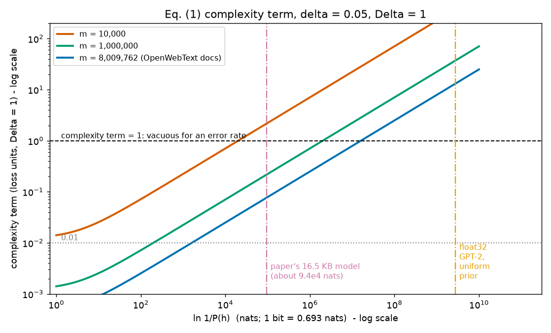
The figure shows the same curve for three dataset sizes. On log-log axes each curve becomes a straight line of slope one half once the price dominates \(\ln(1/\delta)\). Multiplying \(m\) by 100 moves the line down by a factor 10.
(b) Turned around: how large a price can we afford?¶
Setting the complexity term equal to a target \(\varepsilon\) and solving for the price (deeper block "Solving for the budget") gives
Script section [3]:
| target | \(\Delta\) | largest \(\ln(1/P(h))\) (nats) | bits | KB (8,192 bits) |
|---|---|---|---|---|
| 0.01 (fraction) | 1 | 1,599.0 | 2,307 | 0.28 |
| 0.1 (fraction) | 1 | 160,192.2 | 231,109 | 28.21 |
| 2 bits/token | 18.787 | 181,547.0 | 261,917 | 31.97 |
| 1 bit/token | 18.787 | 45,384.5 | 65,476 | 7.99 |
So, at OpenWebText's size, a model whose prior price is a few tens of kilobytes can have a complexity term of a couple of bits per token. A non-vacuous bits-per-token bound needs the empirical risk plus this term to stay below 15.617. Chapter 14 turns these budgets into compressed sizes.
(c) What matters and what hardly does¶
Script section [4] varies \(\delta\) and \(m\) (with \(\Delta = 1\)).
| \(\delta\) | \(\ln(1/\delta)\) (nats) | term at price 10 nats | term at price 100,000 nats |
|---|---|---|---|
| 0.1 | 2.303 | 0.000876 | 0.079010 |
| 0.05 | 2.996 | 0.000901 | 0.079010 |
| 0.01 | 4.605 | 0.000955 | 0.079011 |
| 0.001 | 6.908 | 0.001027 | 0.079011 |
| 0.000001 | 13.816 | 0.001219 | 0.079014 |
- Confidence is cheap. Going from 95 % to 99.9999 % confidence adds 10.82 nats to the price (\(13.816 - 2.996\); script section [4]). Next to a price of 100,000 nats this changes the term in the sixth digit. The choice of \(\delta\) matters only for very cheap hypotheses.
- Data are expensive. At a price of 100,000 nats the term is 2.23610 for \(m\) = 10,000, 0.22361 for 1,000,000, 0.07901 for 8,009,762 and 0.02236 for 100,000,000. That is the \(1/\sqrt m\) law.
(d) Counting versus weighting at the paper's scale¶
Script section [5].
- Uniform prior (counting). Float32 GPT-2 small, \(D = 123{,}689{,}472\) parameters, \(\ln\lvert\mathcal H\rvert = 32D\ln 2 = 2.7435\times10^{9}\) nats. Complexity term: 13.0867 for \(\Delta = 1\), and 245.86 bits/token for \(\Delta = 18.787\). Both vacuous; these reproduce Chapter 10's numbers.
- Weighting by compressed size. The paper's best bits-per-token model compresses to 16.5325 KB, read from Fig. 2
(p. 5) by
fig_extract.py(erratum §F; 1 KB = 8,192 bits, erratum E35). That is 135,434.26 bits. Chapters 12–14 explain why a model of \(C\) bits may be given a prior with \(\ln(1/P(h)) = C\ln 2 + 2\ln C\). Here that is 93,899.5 nats, \(3.42\times10^{-5}\) of the counting price. The model uses smoothing weight 0.25, for which the interval width is 17.2020 bits per token. Eq. (1) then gives a complexity term of 1.3170 bits per token.
This last number is not yet the paper's: Eq. (1) assumes the training risk is computed on all \(m\) documents, and it ignores the bits needed to name the chosen hyperparameters. Chapter 14 adds those bits and Chapter 17 the cost of estimating the risk on a subsample. The full calculation reproduces Table 1's 12.12 bits per token (erratum §F).
A further point from script section [5]: if you cannot decide between two priors \(P_1\) and \(P_2\), use their average \(P = (P_1 + P_2)/2\). It is fixed in advance and adds up to at most 1, and for every \(h\), \(\ln(1/P(h)) \le \ln 2 + \ln(1/P_i(h))\) for both \(i\). Hedging costs at most \(\ln 2 = 0.6931\) nats, one bit.
(e) Checking the theorem by simulation, and the cheating prior¶
Script sections [6] and [7] run Theorem A.1 on a toy problem in which every true risk is known exactly.
Data. Each example is a number \(z\) drawn uniformly from \([0, 1]\) with a label \(y \in \{0,1\}\). The clean label is \(1\) when \(z \ge 0.3\); then it is flipped with probability 0.2 (label noise). The loss is the 0-1 loss, so \(\Delta = 1\). Each run draws \(m = 200\) examples; there are 10,000 independent runs.
Hypothesis space, fixed before any data:
- 1,023 thresholds "predict 1 if \(z \ge k/1024\)", for \(k = 1,\dots,1023\). The true risk of the threshold \(\theta\) is \(0.2 + 0.6\,\lvert\theta - 0.3\rvert\); the best one in the space has true risk 0.2001.
- \(2^{64}\) lookup tables: cut \([0,1]\) into 64 equal cells and store one predicted label per cell. A lookup table can fit noise that a threshold cannot.
Prior, fixed before any data. Half of the weight goes to thresholds, half to lookup tables. A threshold whose binary expansion needs \(j\) digits (for example \(1/4\) needs 2 and \(5/16\) needs 4; we call \(j\) its level) gets weight \(2^{-2j}\), so coarse thresholds are cheap. Every lookup table gets \(2^{-65}\). The weights add up to 0.999512. The prices are 2.773 nats for a level-2 threshold, 13.863 for a level-10 threshold and 45.055 for any lookup table.
Two training rules.
- ERM: return the hypothesis with the smallest training error (empirical risk minimization, Chapter 10). It picks a lookup table in 96.84 % of runs, because a table can fit some of the noise.
- Minimize the bound: return the hypothesis with the smallest right-hand side of Eq. (1). This rule, which trades training error against price, is known as structural risk minimization. It always picks a threshold, mostly of level 2 (60.25 % of runs) or level 4 (34.38 %).
Three ways of computing the margin. The honest prior above; the uniform prior over all of \(\mathcal H\) (\(\ln\lvert\mathcal H\rvert = 44.361\) nats, margin 0.3441 for everyone); and the cheating prior, \(P(\hat h) = 1\) after training (margin 0.0865).
| rule (means over 10,000 runs) | \(\hat R(\hat h)\) | \(R(\hat h)\) | gap | bound, prior | bound, uniform | fails, prior | fails, uniform | fails, cheat |
|---|---|---|---|---|---|---|---|---|
| ERM | 0.1716 | 0.3033 | 0.1317 | 0.5136 | 0.5157 | 0.0000 | 0.0000 | 0.9357 |
| minimize the bound | 0.2143 | 0.2231 | 0.0088 | 0.3442 | 0.5584 | 0.0004 | 0.0000 | 0.0025 |
"Fails" is the fraction of runs in which \(R(\hat h)\) exceeds the bound.
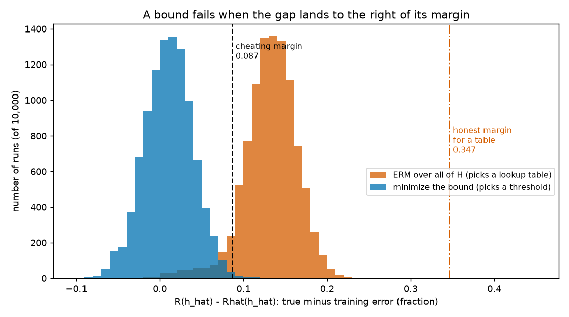
What to notice:
- The theorem holds. With the prior fixed in advance, the bound fails in 0.0000 (ERM) and 0.0004 (bound minimizer) of runs, far below the allowed 0.05. Hoeffding's inequality and the union bound are both loose here (Chapters 9 and 10 measured how loose).
- The cheating prior fails badly with ERM. Its margin 0.0865 is the single-hypothesis Hoeffding margin. ERM's lookup tables have a true-minus-training gap of 0.1317 on average, and the gap is below 0.0865 in fewer than 5 % of runs (its 5 % quantile is 0.0794). The cheat fails in 93.57 % of runs.
- With weak selection, the cheat often gets away with it. The bound-minimizer chooses among a few cheap thresholds, so its selection effect is small, and the cheat fails in only 0.25 % of runs. That is luck, not a guarantee: nothing in the cheat's reasoning distinguishes the two rules.
- Weighting beats counting when training lands on a cheap hypothesis. For the bound-minimizer, the prior gives an average bound of 0.3442; the uniform prior 0.5584. For ERM, which lands on expensive tables, the prior's bound (0.5136) is no better than counting (0.5157).
- The bound rewards the right choice. The bound-minimizer's true risk, 0.2231, is close to the best possible 0.2001. ERM's lookup tables have true risk 0.3033 although their training error looks better.
Going deeper¶
Everything in this section is MY EXPLANATION unless tagged.
The six blocks below prove Theorem A.1 line by line, solve for the budget, handle edge cases (including the per-hypothesis width of erratum E49 above), analyse data-dependent priors, discuss how to choose a prior, and relate Eq. (1) to PAC-Bayes.
Going deeper: Theorem A.1, proved line by line
PAPER §A.1, pp. 12–13 The paper's proof has four displayed steps: Hoeffding for a fixed \(h\); the choice of \(t(h)\); solving for \(t(h)\) (Eq. 6); the union over all \(h\). MY EXPLANATION We follow it and fill in every step.
Setting. Everything listed in the theorem box is fixed before the data. The documents \(X_1,\dots,X_m\) are i.i.d. For each \(h\in\mathcal H\), write \(Z_j(h) = R(h, X_j)\) for its loss on document \(j\) (loss units).
Step 1: one fixed hypothesis. Fix \(h\in\mathcal H\). The numbers \(Z_1(h),\dots,Z_m(h)\) are functions of independent documents through one fixed function, so they are independent. Each lies in \([a, a+\Delta]\). Their average is \(\hat R(h)\), and its expected value is \(R(h)\). For any \(t > 0\),
Line 1 multiplies both sides of the inequality by \(m > 0\), which does not change the event. Line 2 rewrites it with \(\sum_j Z_j(h) = m\hat R(h)\) and \(\mathbb E\sum_j Z_j(h) = mR(h)\). Line 3 is the lower-tail Hoeffding inequality of Chapter 9 for a sum of \(m\) independent terms, each of width \(\Delta\), with deviation \(\varepsilon = mt\); the sum of squared widths is \(m\Delta^2\). The probability is over the documents; \(h\), \(R(h)\), \(t\), \(m\), \(\Delta\) are fixed.
Step 2: choose the margin. The paper chooses \(t(h)\) separately for each \(h\) so that the right side equals \(h\)'s share of the budget:
This needs \(P(h) > 0\) (for \(P(h) = 0\) see the edge-cases block). Both sides are positive, so take \(\ln\) of both:
The middle step is the product rule for logarithms; the last uses \(\ln x = -\ln(1/x)\). Multiply both sides by \(-\Delta^2/(2m)\):
The right side is positive, because \(P(h)\le 1\) and \(\delta < 1\) make both logarithms at least 0 and the second strictly positive. Take the positive square root:
This is the paper's Eq. (6). Units: the two logarithms are pure numbers (nats), \(m\) is a count, so \(t(h)\) has the units of \(\Delta\). Section [1] of the script checks that this \(t(h)\) satisfies the defining equation to \(10^{-9}\).
Step 3: the union. Define the bad event \(E_h = \{R(h) \ge \hat R(h) + t(h)\}\) for each \(h\in\mathcal H\). By Steps 1 and 2, \(\Pr[E_h] \le P(h)\delta\). By the union bound (Chapter 10),
The paper writes the last step as "\(=\delta\)", which holds when the weights add up to exactly 1 (erratum E50).
Step 4: complement. With probability at least \(1-\delta\), no \(E_h\) happens, so \(R(h) < \hat R(h) + t(h)\) for every \(h\in\mathcal H\) at once. (A strict "\(<\)" is slightly stronger than the theorem's "\(\le\)".)
Step 5: the trained hypothesis. \(\hat h\) is some member of \(\mathcal H\), whatever the data. If its bound fails, then the bad event of the hypothesis it turned out to be has happened: \(\{R(\hat h) \ge \hat R(\hat h) + t(\hat h)\} \subseteq \bigcup_h E_h\). So \(\Pr[R(\hat h) \ge \hat R(\hat h) + t(\hat h)] \le \delta\). This is the paper's last display, with \(h^*\) for our \(\hat h\). \(\square\)
Why Step 1 alone is not enough. The paper notes that \(\hat R(\hat h)\) is not an average of independent variables, because \(\hat h\) was built from the same documents. Step 1 therefore cannot be applied to \(\hat h\) directly. Steps 3–5 avoid this: Hoeffding is only ever applied to fixed, listed hypotheses.
What \(R(\hat h)\) means. The theorem defines \(R(h) = \mathbb E[\hat R(h)]\) for a fixed \(h\). For the trained hypothesis, \(R(\hat h)\) is that function evaluated at the random point \(\hat h\) (hold \(\hat h\) fixed, average its loss over a fresh document). It is not \(\mathbb E[\hat R(\hat h)]\), which selection pushes down (Chapter 10).
Going deeper: solving for the budget, and the cost of confidence
Budget. Fix a target \(\varepsilon > 0\) (loss units). The complexity term is at most \(\varepsilon\) exactly when
The first equivalence divides by \(\Delta > 0\) and squares (both sides are non-negative, and squaring is increasing on non-negative numbers). The second multiplies by \(2m\) and subtracts \(\ln(1/\delta)\). In bits, divide the right side by \(\ln 2\). Section [3] of the script checks each budget by plugging it back in.
Equivalent data requirement. Solving the same inequality for \(m\): \(m \ge \Delta^2(\ln(1/P(h)) + \ln(1/\delta))/(2\varepsilon^2)\). The data needed grows linearly in the price.
The cost of confidence. Write \(c = \ln(1/P(h))\) and \(\ell = \ln(1/\delta)\). Changing \(\delta\) changes the term by the factor \(\sqrt{(c + \ell')/(c + \ell)}\). For \(c\) much larger than \(\ell\) and \(\ell'\), this is close to \(1 + (\ell' - \ell)/(2c)\) (first-order expansion of \(\sqrt{1+x}\) around \(x = 0\)). At \(c = 100{,}000\) nats and \(\ell' - \ell = 10.82\) nats the factor is about \(1 + 5.4\times10^{-5}\) (script section [4]), which matches the script's ratio 1.00005. At \(c = 10\) nats the factor is 1.35372 (script section [8]).
Going deeper: edge cases, including per-hypothesis widths
Per-hypothesis intervals. Suppose hypothesis \(h\) has its own interval \([a(h), a(h)+\Delta(h)]\), fixed before the data (for example because a smoothing weight \(\alpha\) is part of \(h\) and sets \(\Delta(\alpha)\); Chapter 16). Step 1 of the proof concerns a single fixed \(h\), so Hoeffding gives \(\Pr[R(h) \ge \hat R(h) + t] \le \exp(-2mt^2/\Delta(h)^2)\). Step 2 then gives \(t(h) = \Delta(h)\sqrt{(\ln(1/P(h)) + \ln(1/\delta))/(2m)}\). Steps 3–5 never mention \(\Delta\). So, with probability at least \(1-\delta\), \(R(h) \le \hat R(h) + \Delta(h)\sqrt{(\ln(1/P(h)) + \ln(1/\delta))/(2m)}\) for every \(h\) at once. What must not happen is a width chosen after looking at the data for a given \(h\); that would break Step 1 as a data-dependent prior breaks Step 2.
Weights adding up to less than 1. Step 3 ends with \(\delta\sum_h P(h) \le \delta\). Nothing else changes. Unused weight is unused budget.
Zero weight. If \(P(h) = 0\), set \(t(h) = +\infty\). The bad event "\(R(h) \ge \hat R(h) + \infty\)" is impossible, so it contributes 0 to the sum and the proof goes through. The certificate for such an \(h\) is empty.
Countably many hypotheses. The union bound holds for endless lists (Chapter 10), and so does Step 3, provided \(\sum_h P(h) \le 1\). Only the theorem's word "finite" is stronger than needed; Chapter 10 showed that equal weights are impossible for an endless list, so a prior is then not a luxury but a necessity.
The same function listed twice. In the toy, a threshold at a multiple of \(1/64\) computes the same predictions as one of the lookup tables. The proof works for any list of hypotheses, with repeats; a repeated function just receives two shares of the budget, and either of its two margins is valid.
\(\hat h\) must lie in \(\mathcal H\) for every possible dataset. Step 5 needs this. If training could return something outside the list (for example a model stored at higher precision than the class assumes), the certificate does not cover it.
Two-sided version. To bound \(\lvert R(h) - \hat R(h)\rvert\), give each \(h\) two bad events (one per tail), each with share \(P(h)\delta/2\). The margin becomes \(\Delta\sqrt{(\ln(1/P(h)) + \ln(2/\delta))/(2m)}\).
Going deeper: data-dependent priors, the cheat and the legal versions
Where the cheat breaks the proof. Let the weights \(P_S(h)\) depend on the training set \(S\), and set \(t_S(h)\) from them. For a listed \(h\), the event \(\{R(h) \ge \hat R(h) + t_S(h)\}\) now involves two random quantities, \(\hat R(h)\) and \(t_S(h)\), that depend on the same documents. Step 1 needs a fixed margin, so it no longer applies. Nothing else in the proof can repair this.
The cheating prior concretely. With \(P_S(\hat h_S) = 1\) the price is 0, and the margin is \(\Delta\sqrt{\ln(1/\delta)/(2m)}\): the margin of one hypothesis fixed in advance, used for a selected one. In the toy (\(m = 200\)) this is 0.0865, and ERM's lookup tables beat it in 93.57 % of runs (script section [7]).
A milder cheat is still a cheat. Giving the trained model weight \(1/2\) after training and spreading the rest over \(\mathcal H\) also adds up to 1, and also breaks Step 1. Any rule that looks at the training set before fixing the weights is outside the theorem, whatever the resulting numbers look like.
Legal data-dependent priors. A prior may depend on data that are independent of the training set. Condition on those other data: given them, the prior is a fixed rule, and the theorem applies to the training set (the law of total probability of Chapter 1 then removes the conditioning). SOURCE: Lotfi et al. 2022, §5.2 Lotfi et al. (2022) study such priors, learned on one part of the data and evaluated on another. MY EXPLANATION The paper's own priors are fixed in advance: they depend only on the architecture, the hyperparameter grid and the compression scheme (Chapters 13, 14 and 24).
Choosing the hyperparameters after seeing the data. That is a selection, not a change of prior. It is legal if every option was given its own weight in advance; the paper pays \(\log_2\) of the number of options in bits (Chapter 24). Erratum E07 concerns one place where a selection is not paid for in the second term of the subsampling bound (Chapter 17).
Going deeper: how to choose a prior
The ideal prior, in hindsight. If we knew which \(h\) training would return, giving it weight 1 would make the price 0. We do not, and choosing after the fact is the cheat. The best one can do in advance is to concentrate weight on the hypotheses training is likely to return.
No free lunch. Because the weights add up to at most 1, at most \(2^k\) hypotheses can have weight at least \(2^{-k}\), that is a price of at most \(k\) bits. (If more than \(2^k\) had weight at least \(2^{-k}\), the weights would add up to more than 1.) A prior can make a few hypotheses cheap, never all of them.
Mixtures. If \(P_1,\dots,P_K\) are priors fixed in advance, so is \(P = \frac1K\sum_i P_i\), and \(P(h) \ge P_i(h)/K\) for every \(i\). Hence \(\ln(1/P(h)) \le \ln K + \min_i \ln(1/P_i(h))\): you get the best of \(K\) priors for an extra \(\ln K\) nats. For \(K = 2\) this is \(\ln 2 = 0.6931\) nats, one bit (script section [5]). The toy prior is such a mixture: half on thresholds, half on lookup tables.
Priors from codes. The paper's prior is built from description lengths: a model that can be written down in \(C\) bits gets weight about \(2^{-C}\). Chapter 12 proves that, for a suitable code, such weights add up to at most 1 (the Kraft inequality), Chapter 13 relates them to the shortest possible description (Kolmogorov complexity and the Solomonoff prior), and Chapter 14 turns them into the price \(C\ln 2 + 2\ln C\) nats used in worked example (d). The toy's threshold prior is a small instance: a threshold with \(j\) binary digits costs \(2j\) bits.
Going deeper: Eq. (1) and PAC-Bayes
Posterior and KL divergence. In PAC-Bayes, after seeing the data one chooses a probability distribution \(Q\) over \(\mathcal H\), called the posterior, and predicts by drawing \(h\) from \(Q\). The Kullback–Leibler (KL) divergence from \(P\) to \(Q\) is
(in nats; terms with \(Q(h) = 0\) count as 0). It is 0 when \(Q = P\) and grows as \(Q\) moves its mass to hypotheses the prior considers unlikely.
Point mass. Let \(Q\) put all its mass on one hypothesis \(h_0\): \(Q(h_0) = 1\), \(Q(h) = 0\) otherwise. Then only one term survives:
exactly the price in Eq. (1).
SOURCE: Lotfi et al. 2022, §3, Eq. (2) Lotfi et al. (2022) make the same observation: with a point-mass posterior, the KL term is the log of one over the prior weight. They describe the PAC-Bayes bound of McAllester as the finite-hypothesis bound with \(\ln\lvert\mathcal H\rvert\) replaced by \(\mathrm{KL}(Q\,\Vert\,P)\) and the single hypothesis replaced by a random draw from \(Q\); that bound reads \(\mathbb E_{h\sim Q}[R(h)] \le \mathbb E_{h\sim Q}[\hat R(h)] + \sqrt{(\mathrm{KL}(Q\Vert P) + \ln(m/\delta) + 2)/(2m-1)}\) for a loss in \([0,1]\), written here with \(m\) examples.
MY EXPLANATION Two consequences.
- For a point mass, this PAC-Bayes bound is slightly looser than Eq. (1): it pays \(\ln(m/\delta) + 2\) instead of \(\ln(1/\delta)\) and divides by \(2m-1\) instead of \(2m\). Eq. (1) is the cleaner tool for one deterministic model.
- PAC-Bayes earns its keep when \(Q\) is spread out. A spread-out \(Q\) can have a KL much smaller than \(\ln(1/P(h))\) for any single \(h\) it contains, but then the certified object is a randomly drawn model, not the trained one. With continuous parameters and a continuous prior, a point mass has infinite KL, which is why PAC-Bayes bounds for neural networks usually add noise to the weights. The paper's models are discrete (quantized, Chapter 21), so a point mass is affordable.
No PAC-Bayes bound is derived in this explainer; we only need the comparison.
Going deeper: the toy experiment in detail
Exact true risks. For the threshold \(\theta\), the clean label disagrees with the prediction on an interval of length \(\lvert\theta - 0.3\rvert\). There the prediction is wrong unless the label was flipped (probability 0.8 of an error); elsewhere it is right unless the label was flipped (probability 0.2). So \(R = 0.2(1 - \lvert\theta - 0.3\rvert) + 0.8\lvert\theta - 0.3\rvert = 0.2 + 0.6\lvert\theta - 0.3\rvert\). A lookup table's risk is the same calculation cell by cell, averaged over the 64 cells.
Prior. Level \(j\) (\(j = 1,\dots,10\)) contains the \(2^{j-1}\) thresholds \(k/2^j\) with \(k\) odd. Each gets \(2^{-2j}\), so level \(j\) in total gets \(2^{j-1}\cdot2^{-2j} = 2^{-j-1}\), and all thresholds together get \(\sum_{j=1}^{10}2^{-j-1} = \frac12(1 - 2^{-10})\). The \(2^{64}\) tables get \(2^{-65}\) each, \(\frac12\) in total. Sum: \(1 - 2^{-11} = 0.999512\), as printed.
Training rules. ERM breaks ties in favour of thresholds, then the smallest \(k\); a lookup table fits each cell by majority vote (ties and empty cells predict 0). The bound minimizer compares the best threshold bound with the best lookup-table bound; all tables have the same price, so the best table is the ERM table.
Why ERM's tables generalize badly. With 200 examples and 64 cells, a cell holds 3.125 examples on average. A majority of 3 noisy labels is wrong with noticeable probability, and the training error counts only the minority labels. The resulting gap, 0.1317 on average, is selection bias in action.
Common misconceptions¶
Everything in this section is MY EXPLANATION.
- Misconception: The prior must be the true distribution of hypotheses, or at least an honest belief. — Actually: any weights fixed before the data, adding up to at most 1, give a valid bound. A prior that favours the wrong hypotheses gives a loose bound, never a false one.
- Misconception: The bound gets worse when the hypothesis space gets bigger. — Actually: Eq. (1) depends on the space only through \(P(\hat h)\). The toy space has more than \(2^{64}\) members, yet a level-2 threshold pays 2.773 nats. This is why the paper can certify models whose architectures have hundreds of millions of parameters.
- Misconception: Any weights that add up to 1 are a valid prior, even if chosen after training. — Actually: the weights must be fixed before the training data are seen. Putting weight 1 on the trained hypothesis after the fact made the "bound" fail in 93.57 % of runs in worked example (e).
- Misconception: Demanding more confidence (smaller \(\delta\)) makes the bound much looser. — Actually: \(\delta\) enters through \(\ln(1/\delta)\). Going from \(\delta = 0.05\) to \(10^{-6}\) changes the term at a price of 100,000 nats from 0.079010 to 0.079014.
- Misconception: Eq. (1) is a statement about a model drawn at random from the prior. — Actually: the prior is bookkeeping for the failure budget. The certified object is the one deterministic model \(\hat h\) that training returned. Bounds about randomly drawn models are PAC-Bayes bounds.
- Misconception: The "log" in Eq. (1) can be read as \(\log_2\) because the paper measures sizes in bits. — Actually: it must be \(\ln\) (erratum E02); a size in bits must be multiplied by \(\ln 2\) first.
Self-test¶
Q1. A model is assigned prior weight \(P(h) = 2^{-10{,}000}\). Using \(m = 8{,}009{,}762\) documents SOURCE: nanoGPT; erratum E32 and \(\delta = 0.05\) SOURCE: authors' code; erratum E31, compute the complexity term of Eq. (1) for a top-1 error (\(\Delta = 1\)) and for smoothed bits per token with \(\Delta = 18.787\).
Answer
The price is \(\ln(1/P(h)) = 10{,}000\ln 2 = 6{,}931.47\) nats (convert bits to nats before using Eq. 1; erratum E02). Then the term is \(\sqrt{(6{,}931.47 + 2.9957)/(2\times8{,}009{,}762)} = 0.02081\) for \(\Delta = 1\), and \(18.787\times0.02081 = 0.3909\) bits per token for \(\Delta = 18.787\) (script section [8]). Ten thousand bits of description cost about 2 percentage points of top-1 error at this dataset size.
Q2. A colleague trains a model, sees that it is the 37th hypothesis on a pre-registered list of 1,000, and then proposes the prior "weight 0.9 on hypothesis 37, the remaining 0.1 spread evenly over the other 999". The weights add up to 1. Is the resulting bound valid? What should they have done instead?
Answer
No. The weights were chosen after seeing which hypothesis training returned, so they are random, and Step 1 of the proof (Hoeffding for a fixed margin) does not apply. The fact that they add up to 1 is irrelevant; the cheating prior of worked example (e) also adds up to 1 and failed in 93.57 % of runs. Valid alternatives: use a prior fixed before training (for example uniform over the 1,000, which is the Occam bound with price \(\ln 1000\)), or a prior fixed in advance that favours hypotheses expected to do well. If they had reasons to favour hypothesis 37 before training, they should have written those weights down then.
Q3. For a hypothesis with price 100,000 nats, by what factor does the complexity term change when \(\delta\) goes from 0.05 to \(10^{-6}\)? And for price 10 nats? Explain the difference.
Answer
The term is proportional to \(\sqrt{c + \ln(1/\delta)}\) with \(c\) the price. \(\ln 20 = 2.996\) and \(\ln 10^6 = 13.816\) nats. At \(c = 100{,}000\) the factor is \(\sqrt{100{,}013.816/100{,}002.996} = 1.00005\) (term 0.079010 to 0.079014). At \(c = 10\) it is \(\sqrt{23.816/12.996} = 1.35372\) (0.000901 to 0.001219) (script section [8]). When the price dominates, confidence is nearly free; for very cheap hypotheses the \(\ln(1/\delta)\) part is a large share of the total.
Code for this chapter¶
Run it from the project root:
.venv/Scripts/python explainer/code/ch11_eq1_calculator.py
Source: ch11_eq1_calculator.py
"""Chapter 11 demo: an Eq. (1) / Theorem A.1 calculator and a coverage check.

Claims reproduced / illustrated
  * Eq. (1) (paper §4.1, p. 4) = Eq. (5) (App. A.1, p. 12):
        R(h) <= Rhat(h) + Delta * sqrt((ln 1/P(h) + ln 1/delta) / (2m)),
    with the paper's bare "log" read as ln (erratum E02). Computed with pacbound.eq1_complexity.
  * Eq. (6): t(h) solves exp(-2 m t^2 / Delta^2) = P(h) * delta (checked numerically).
  * Tables of the complexity term over ln 1/P(h), m, delta and Delta, with
    m = 8,009,762 documents [SOURCE nanoGPT / authors' code, erratum E32] and
    delta = 0.05 [SOURCE authors' code, erratum E31]; Delta = 1 (top-k error, fraction) and
    Delta(alpha = 0.1) = 18.787 bits/token (Theorem A.2, pacbound.smoothing_interval; Ch. 16).
  * Inverse use: the largest ln 1/P(h) that keeps the complexity term below a target.
  * Uniform prior P = 1/|H| gives the Occam bound (Ch. 10): float32 GPT-2 small is vacuous.
  * Scale of the paper's best model under Eq. (1) alone: compressed size 16.5325 KB, alpha = 0.25
    (read from Fig. 2 by fig_extract.py; 1 KB = 8192 bits, erratum E35).
  * Coverage simulation of Theorem A.1 on a toy finite class (thresholds + lookup tables) with
    a prior fixed before the data: the bound fails in far fewer than delta of the runs.
  * "Cheating prior": putting all prior mass on the trained hypothesis AFTER seeing the data
    makes Eq. (1) fail far more often than delta.

Outputs: code/outputs/ch11_eq1_calculator.txt,
         docs/assets/fig/ch11_complexity_curve.png, docs/assets/fig/ch11_cheating_prior.png
"""
from __future__ import annotations

import json
import math
import sys
import time
from pathlib import Path

import numpy as np

import matplotlib
matplotlib.use("Agg")
import matplotlib.pyplot as plt

HERE = Path(__file__).resolve().parent
sys.path.insert(0, str(HERE))
import pacbound as pb  # noqa: E402

OUT_TXT = HERE / "outputs" / "ch11_eq1_calculator.txt"
FIG_DIR = HERE.parent / "docs" / "assets" / "fig"
FIG1 = FIG_DIR / "ch11_complexity_curve.png"
FIG2 = FIG_DIR / "ch11_cheating_prior.png"

M = pb.M_DOCS              # 8,009,762 documents [SOURCE]
DELTA = pb.DELTA           # 0.05 [SOURCE]
LN2 = pb.LN2

# toy coverage simulation -------------------------------------------------------
M_TOY = 200                # training examples per run
REPS = 10_000              # independent runs
CHUNK = 2_000              # runs processed at once (memory)
ETA = 0.2                  # label-noise rate
THETA_STAR = 0.3           # clean labels: y = 1[z >= 0.3]
NBIN = 1024                # threshold grid k/1024, k = 1..1023
LEVELS = 10                # 1024 = 2^10
G = 64                     # lookup tables: 64 equal cells, one bit each
BINS_PER_CELL = NBIN // G

lines: list[str] = []


def out(s: str = "") -> None:
    print(s)
    lines.append(s)


def complexity(lnp: float, m: int = M, delta: float = DELTA, width: float = 1.0) -> float:
    """Second term of Eq. (1), loss units (wrapper around pacbound.eq1_complexity)."""
    return pb.eq1_complexity(lnp, m, delta, width)


def budget(eps: float, m: int = M, delta: float = DELTA, width: float = 1.0) -> float:
    """Largest ln 1/P(h) (nats) with complexity term <= eps:  2 m eps^2 / width^2 - ln(1/delta)."""
    return 2.0 * m * eps * eps / (width * width) - math.log(1.0 / delta)


def threshold_levels() -> np.ndarray:
    """Dyadic level j of k/1024 for k = 1..1023: k = 2^a * odd  ->  j = 10 - a (1..10)."""
    ks = np.arange(1, NBIN)
    a = np.zeros_like(ks)
    kk = ks.copy()
    while np.any(kk % 2 == 0):
        even = kk % 2 == 0
        a[even] += 1
        kk[even] //= 2
    return LEVELS - a


def main() -> None:
    t0 = time.time()
    OUT_TXT.parent.mkdir(parents=True, exist_ok=True)
    FIG_DIR.mkdir(parents=True, exist_ok=True)

    out("Chapter 11 - Eq. (1) calculator and Theorem A.1 coverage  (ch11_eq1_calculator.py)")

    # [1] inputs ----------------------------------------------------------------
    lo, hi, d01 = pb.smoothing_interval(0.1)
    lo25, hi25, d25 = pb.smoothing_interval(0.25)
    out("[1] Inputs")
    out(f"  m = {M:,} documents [SOURCE nanoGPT/authors' code];  delta = {DELTA} [SOURCE authors' code]")
    out(f"  ln(1/delta) = ln 20 = {math.log(1 / DELTA):.6f} nats;  ln 2 = {LN2:.6f} nats per bit")
    out(f"  Delta = 1 (top-k error, fraction);  Delta(alpha=0.1) = {d01:.3f} bits/token;"
        f"  log2 V = {pb.random_guess_bpd():.3f} bits/token")
    # Eq. (6) check: exp(-2 m t^2/Delta^2) = P(h) delta
    for lnp in (10.0, 1e5):
        t = complexity(lnp, width=d01)
        lhs_exponent = 2.0 * M * t * t / (d01 * d01)          # -ln of Hoeffding's right side
        rhs_exponent = lnp + math.log(1.0 / DELTA)             # -ln (P(h) delta)
        assert abs(lhs_exponent - rhs_exponent) < 1e-9 * rhs_exponent
        if lnp < 700:
            assert abs(pb.hoeffding_tail(t, M, d01) / (math.exp(-lnp) * DELTA) - 1) < 1e-9
    out("  (checked: t(h) of Eq. (6) satisfies exp(-2 m t^2/Delta^2) = P(h) delta to 1e-9)")

    # [2] the calculator table ---------------------------------------------------
    out()
    out("[2] Complexity term Delta*sqrt((ln 1/P(h) + ln 1/delta)/(2m)), m = 8,009,762, delta = 0.05")
    out("   ln 1/P(h) [nats]   = bits      | Delta = 1 (fraction) | Delta = 18.787 (bits/token)")
    table = [0.0, 10.0, 1e3, 1e4, 1e5, 1e6, 1e7]
    for lnp in table:
        c1 = complexity(lnp)
        cb = complexity(lnp, width=d01)
        flag1 = "  vacuous" if c1 >= 1 else ""
        flagb = "  vacuous" if cb >= pb.random_guess_bpd() else ""
        out(f"   {lnp:>14,.0f}  {lnp / LN2:>13,.0f}  | {c1:>10.5f}{flag1:<9} | {cb:>10.4f}{flagb}")
    assert abs(complexity(0.0) - pb.hoeffding_t(M, 1.0, math.log(20))) < 1e-15
    out(f"   (1e6 nats = {1e6 / LN2 / 8192:.1f} KB at 8192 bits per KB)")

    # [3] inverse: how much prior surprise can we afford? -----------------------
    out()
    out("[3] Budget: largest ln 1/P(h) with complexity term <= target (m = 8,009,762, delta = 0.05)")
    for eps, w, unit in ((0.01, 1.0, "(fraction)"), (0.1, 1.0, "(fraction)"),
                         (2.0, d01, "bits/token"), (1.0, d01, "bits/token")):
        b = budget(eps, width=w)
        assert abs(complexity(b, width=w) - eps) < 1e-9
        out(f"  target {eps:<4} {unit:<10} Delta = {w:6.3f}: ln 1/P <= {b:>12,.1f} nats"
            f" = {b / LN2:>12,.0f} bits = {b / LN2 / 8192:>8.2f} KB")

    # [4] sensitivity -------------------------------------------------------------
    out()
    out("[4] Sensitivity, Delta = 1 (complexity term at ln 1/P(h) = 10 and = 100,000 nats)")
    for dl in (0.1, 0.05, 0.01, 1e-3, 1e-6):
        out(f"  delta = {dl:<7g} ln(1/delta) = {math.log(1 / dl):6.3f} nats   ln1/P=10: "
            f"{complexity(10.0, delta=dl):.6f}   ln1/P=1e5: {complexity(1e5, delta=dl):.6f}")
    dl_cost = math.log(1e6) - math.log(20)
    out(f"  95% -> 99.9999% confidence adds ln(1e6) - ln(20) = {dl_cost:.2f} nats;"
        f" first-order factor at 1e5 nats: 1 + {dl_cost / 2e5:.1e}")
    out("  ln1/P=1e5, varying m: " + ";  ".join(
        f"m = {mm:,}: {complexity(1e5, m=mm):.5f}" for mm in (10_000, 1_000_000, M, 100_000_000)))

    # [5] uniform prior = Occam bound; the paper's scale ---------------------------
    out()
    out("[5] Uniform prior P = 1/|H| (Occam bound, Ch. 10) vs a weighting prior")
    D = pb.gpt2_params(12, 768)
    assert D == 123_689_472
    ln_h = 32 * D * LN2
    out(f"  float32 GPT-2 small: D = {D:,}; ln|H| = 32 D ln 2 = {ln_h:.4e} nats;"
        f" complexity, Delta = 1: {complexity(ln_h):.4f}   Delta = 18.787: "
        f"{complexity(ln_h, width=d01):.2f} bits/token  (vacuous)")
    # Fig. 2 (left), best BPD model, exact value read from the PDF by fig_extract.py (same as ch14/ch17)
    _fig = json.loads((HERE / "outputs" / "fig_extract.json").read_text(encoding="utf-8"))["figure2"]["left"]
    _i = min(range(len(_fig["bound"])), key=lambda i: _fig["bound"][i]["value"])
    kb = _fig["compressed_size_kb"][_i]["value"]
    c_bits = kb * 8192
    lnp_paper = pb.log_inv_prior_nats_from_bits(c_bits)
    assert abs(c_bits - 135_434.26) < 0.01 and abs(lnp_paper - 93_899.5) < 0.05
    out(f"  paper's best BPD model (Fig. 2): C = {kb:.4f} KB = {c_bits:,.2f} bits (1 KB = 8192 bits);"
        f" ln 1/P = C ln2 + 2 ln C = {lnp_paper:,.1f} nats  (= {lnp_paper / ln_h:.2e} of float32 ln|H|)")
    out(f"    Eq. (1) complexity, Delta(alpha=0.25) = {d25:.4f} bits/token: "
        f"{complexity(lnp_paper, width=d25):.4f} bits/token (full data, no hyperparameter bits)")
    out(f"  hedging between two priors, P = (P1 + P2)/2, costs at most ln 2 = {LN2:.4f} nats = 1 bit")

    # [6] + [7] coverage simulation --------------------------------------------------
    out()
    out(f"[6] Coverage of Theorem A.1 on a toy class: m = {M_TOY}, {REPS:,} runs, delta = {DELTA}")
    out(f"  data: z ~ Uniform[0,1], y = 1[z >= {THETA_STAR}] flipped with prob. {ETA};"
        f"  H = 1,023 thresholds k/1024  +  2^{G} lookup tables (one bit per cell of width 1/{G})")
    lev = threshold_levels()                               # level j per threshold
    lnp_thr = 2 * lev * LN2                                # P = 2^(-2j)
    lnp_tab = (G + 1) * LN2                                # P = 2^(-65)
    total_prior = float(np.sum(2.0 ** (-2.0 * lev))) + 0.5
    out(f"  prior (fixed before data): threshold at level j gets 2^(-2j) [ln 1/P = 2j ln 2];"
        f" each table 2^(-{G + 1})")
    out(f"    total prior mass = {total_prior:.6f} (<= 1);  ln 1/P: level 2 = {4 * LN2:.3f},"
        f" level 10 = {20 * LN2:.3f}, table = {lnp_tab:.3f} nats")
    ln_h_toy = G * LN2 + math.log1p(1023 / 2.0 ** G)
    t_cheat = complexity(0.0, m=M_TOY)
    t_tab = complexity(lnp_tab, m=M_TOY)
    t_unif = complexity(ln_h_toy, m=M_TOY)
    out(f"  margins (Delta = 1): cheat (ln 1/P = 0) {t_cheat:.4f}; level-2 threshold "
        f"{complexity(4 * LN2, m=M_TOY):.4f}; level-10 threshold {complexity(20 * LN2, m=M_TOY):.4f};"
        f" table {t_tab:.4f}; uniform prior (ln|H| = {ln_h_toy:.3f}) {t_unif:.4f}")

    thetas = np.arange(1, NBIN) / NBIN
    risk_thr = ETA + (1 - 2 * ETA) * np.abs(thetas - THETA_STAR)         # exact true risk
    edges = np.arange(G + 1) / G
    f1 = np.clip((edges[1:] - THETA_STAR) * G, 0.0, 1.0)                  # clean-1 fraction per cell
    margin_thr = np.array([complexity(v, m=M_TOY) for v in lnp_thr])

    rng = np.random.default_rng(0)
    rec = {k: [] for k in ("erm_rhat", "erm_r", "erm_is_tab", "erm_marg", "bm_rhat", "bm_r", "bm_marg", "bm_lev")}
    for start in range(0, REPS, CHUNK):
        nrep = min(CHUNK, REPS - start)
        z = rng.random((nrep, M_TOY))
        clean = (z >= THETA_STAR).astype(np.int64)
        flip = (rng.random((nrep, M_TOY)) < ETA).astype(np.int64)
        y = clean ^ flip
        b = np.minimum((z * NBIN).astype(np.int64), NBIN - 1)
        idx = (np.arange(nrep)[:, None] * NBIN + b).ravel()
        ones = np.bincount(idx, weights=y.ravel(), minlength=nrep * NBIN).reshape(nrep, NBIN)
        alln = np.bincount(idx, minlength=nrep * NBIN).reshape(nrep, NBIN)
        zeros = alln - ones
        c1 = np.cumsum(ones, axis=1)[:, :-1]                 # ones in bins < k, k = 1..1023
        c0 = np.cumsum(zeros, axis=1)[:, :-1]
        z_tot = zeros.sum(axis=1, keepdims=True)
        rhat_thr = (c1 + (z_tot - c0)) / M_TOY                # predict 0 below k/1024, 1 above
        # lookup tables: majority vote per cell (tie or empty -> 0)
        ones_c = ones.reshape(nrep, G, BINS_PER_CELL).sum(axis=2)
        n_c = alln.reshape(nrep, G, BINS_PER_CELL).sum(axis=2)
        zeros_c = n_c - ones_c
        pred = (ones_c > zeros_c).astype(float)
        rhat_tab = np.minimum(ones_c, zeros_c).sum(axis=1) / M_TOY
        mismatch = np.where(pred == 1, 1 - f1[None, :], f1[None, :])
        r_tab = (ETA + (1 - 2 * ETA) * mismatch).mean(axis=1)

        # rule 1: empirical risk minimization over all of H (ties -> threshold, then smallest k)
        k_best = rhat_thr.argmin(axis=1)
        best_thr = rhat_thr[np.arange(nrep), k_best]
        is_tab = rhat_tab < best_thr
        rec["erm_rhat"].append(np.where(is_tab, rhat_tab, best_thr))
        rec["erm_r"].append(np.where(is_tab, r_tab, risk_thr[k_best]))
        rec["erm_is_tab"].append(is_tab)
        rec["erm_marg"].append(np.where(is_tab, t_tab, margin_thr[k_best]))
        # rule 2: minimize the Eq. (1) bound (structural risk minimization)
        bnd_thr = rhat_thr + margin_thr[None, :]
        kb_ = bnd_thr.argmin(axis=1)
        bt = bnd_thr[np.arange(nrep), kb_]
        tab_wins = rhat_tab + t_tab < bt
        rec["bm_rhat"].append(np.where(tab_wins, rhat_tab, rhat_thr[np.arange(nrep), kb_]))
        rec["bm_r"].append(np.where(tab_wins, r_tab, risk_thr[kb_]))
        rec["bm_marg"].append(np.where(tab_wins, t_tab, margin_thr[kb_]))
        rec["bm_lev"].append(np.where(tab_wins, 0, lev[kb_]))
    r = {k: np.concatenate(v) for k, v in rec.items()}

    erm_marg = r["erm_marg"]
    gap_erm = r["erm_r"] - r["erm_rhat"]
    gap_bm = r["bm_r"] - r["bm_rhat"]

    def row(name, rhat, rr, marg, gap):
        fail_honest = float(np.mean(rr > rhat + marg))
        fail_unif = float(np.mean(rr > rhat + t_unif))
        fail_cheat = float(np.mean(rr > rhat + t_cheat))
        out(f"  {name:<22} {rhat.mean():.4f}  {rr.mean():.4f}  {gap.mean():.4f}  "
            f"{(rhat + marg).mean():.4f}  {(rhat + t_unif).mean():.4f}  "
            f"{fail_honest:.4f}   {fail_unif:.4f}   {fail_cheat:.4f}")
        return fail_honest, fail_cheat

    out(f"  best possible true risk in H = {risk_thr.min():.4f} (threshold 307/1024);"
        f"  examples per lookup-table cell on average: {M_TOY / G:.3f}")
    out("  rule (means over runs)   Rhat    R(h)    gap     bound   bound    fail     fail     fail")
    out("                                                   prior   unif.    prior    unif.    cheat")
    f_erm = row("ERM over all of H", r["erm_rhat"], r["erm_r"], erm_marg, gap_erm)
    f_bm = row("minimize the bound", r["bm_rhat"], r["bm_r"], r["bm_marg"], gap_bm)
    levs, cnts = np.unique(r["bm_lev"], return_counts=True)
    desc = ", ".join(f"L{int(lv)}: {c / REPS:.4f}" if lv > 0 else f"table: {c / REPS:.4f}"
                     for lv, c in zip(levs, cnts))
    out(f"  ERM returned a lookup table in {np.mean(r['erm_is_tab']):.4f} of runs;"
        f" bound-minimizer's threshold level (L): {desc}")
    assert f_erm[0] <= DELTA and f_bm[0] <= DELTA          # Theorem A.1 holds
    out()
    out("[7] Cheating prior: P(h_hat) = 1 chosen AFTER seeing the data -> margin "
        f"{t_cheat:.4f} (ln 1/P = 0)")
    out(f"  failure rate with ERM: {f_erm[1]:.4f}   with the bound-minimizer: {f_bm[1]:.4f}"
        f"   (A.1 promises <= {DELTA} only for a prior fixed in advance);"
        f"  ERM gap R - Rhat: mean {gap_erm.mean():.4f}, 5% quantile {np.quantile(gap_erm, 0.05):.4f}")
    assert f_erm[1] > 10 * DELTA

    # [8] self-test numbers --------------------------------------------------------------
    out()
    out("[8] Self-test")
    q1 = 10_000 * LN2
    out(f"  Q1: P(h) = 2^-10000 -> ln 1/P = {q1:,.2f} nats; complexity (Delta = 1) = {complexity(q1):.5f};"
        f" Delta = {d01:.3f}: {complexity(q1, width=d01):.4f} bits/token")
    for lnp in (10.0, 1e5):
        q3a, q3b = complexity(lnp, delta=0.05), complexity(lnp, delta=1e-6)
        out(f"  Q3: ln 1/P = {lnp:>9,.0f} nats: delta 0.05 -> {q3a:.6f}; delta 1e-6 -> {q3b:.6f}"
            f" (ratio {q3b / q3a:.5f})")

    # figures ----------------------------------------------------------------------------
    fig, ax = plt.subplots(figsize=(8.6, 5.2))
    xs = np.logspace(0, 10, 400)
    for mm, col, lab in ((10_000, "#D55E00", "m = 10,000"), (1_000_000, "#009E73", "m = 1,000,000"),
                         (M, "#0072B2", "m = 8,009,762 (OpenWebText docs)")):
        ax.plot(xs, [complexity(x, m=mm) for x in xs], color=col, lw=2.2, label=lab)
    ax.axhline(1.0, color="black", ls="--", lw=1.1)
    ax.text(1.3, 1.12, "complexity term = 1: vacuous for an error rate", fontsize=9)
    ax.axhline(0.01, color="grey", ls=":", lw=1.1)
    ax.text(1.3, 0.0113, "0.01", fontsize=9, color="grey")
    ax.axvline(lnp_paper, color="#CC79A7", ls="-.", lw=1.3)
    ax.text(lnp_paper * 1.25, 2e-3, "paper's 16.5 KB model\n(about 9.4e4 nats)", fontsize=9,
            color="#CC79A7")
    ax.axvline(ln_h, color="#E69F00", ls="-.", lw=1.3)
    ax.text(ln_h * 1.25, 2e-3, "float32\nGPT-2,\nuniform\nprior", fontsize=9, color="#E69F00")
    ax.set_xscale("log")
    ax.set_xlim(0.7, 3e11)
    ax.set_yscale("log")
    ax.set_ylim(1e-3, 200)
    ax.set_xlabel("ln 1/P(h)  (nats; 1 bit = 0.693 nats)  - log scale")
    ax.set_ylabel("complexity term (loss units, Delta = 1) - log scale")
    ax.set_title("Eq. (1) complexity term, delta = 0.05, Delta = 1")
    ax.legend(fontsize=9, loc="upper left")
    fig.tight_layout()
    fig.savefig(FIG1, dpi=130)
    plt.close(fig)

    fig, ax = plt.subplots(figsize=(8.6, 4.8))
    bins = np.linspace(-0.1, 0.45, 56)
    ax.hist(gap_erm, bins=bins, color="#D55E00", alpha=0.75,
            label="ERM over all of H (picks a lookup table)")
    ax.hist(gap_bm, bins=bins, color="#0072B2", alpha=0.75,
            label="minimize the bound (picks a threshold)")
    ax.axvline(t_cheat, color="black", ls="--", lw=1.4)
    ax.text(t_cheat + 0.004, ax.get_ylim()[1] * 0.93, f"cheating margin\n{t_cheat:.3f}", fontsize=9,
            va="top")
    ax.axvline(t_tab, color="#D55E00", ls="-.", lw=1.4)
    ax.text(t_tab + 0.004, ax.get_ylim()[1] * 0.6, f"honest margin\nfor a table\n{t_tab:.3f}",
            fontsize=9, va="top", color="#D55E00")
    ax.set_xlabel("R(h_hat) - Rhat(h_hat): true minus training error (fraction)")
    ax.set_ylabel(f"number of runs (of {REPS:,})")
    ax.set_title("A bound fails when the gap lands to the right of its margin")
    ax.legend(fontsize=9, loc="upper right", bbox_to_anchor=(1.0, 0.45))
    fig.tight_layout()
    fig.savefig(FIG2, dpi=130)
    plt.close(fig)

    out()
    out(f"figures: docs/assets/fig/{FIG1.name}, {FIG2.name}")
    print(f"runtime {time.time() - t0:.1f} s (console only, so the output file is deterministic)")
    OUT_TXT.write_text("\n".join(lines) + "\n", encoding="utf-8")


if __name__ == "__main__":
    main()
Output:
Chapter 11 - Eq. (1) calculator and Theorem A.1 coverage  (ch11_eq1_calculator.py)
[1] Inputs
  m = 8,009,762 documents [SOURCE nanoGPT/authors' code];  delta = 0.05 [SOURCE authors' code]
  ln(1/delta) = ln 20 = 2.995732 nats;  ln 2 = 0.693147 nats per bit
  Delta = 1 (top-k error, fraction);  Delta(alpha=0.1) = 18.787 bits/token;  log2 V = 15.617 bits/token
  (checked: t(h) of Eq. (6) satisfies exp(-2 m t^2/Delta^2) = P(h) delta to 1e-9)

[2] Complexity term Delta*sqrt((ln 1/P(h) + ln 1/delta)/(2m)), m = 8,009,762, delta = 0.05
   ln 1/P(h) [nats]   = bits      | Delta = 1 (fraction) | Delta = 18.787 (bits/token)
                0              0  |    0.00043          |     0.0081
               10             14  |    0.00090          |     0.0169
            1,000          1,443  |    0.00791          |     0.1487
           10,000         14,427  |    0.02499          |     0.4695
          100,000        144,270  |    0.07901          |     1.4844
        1,000,000      1,442,695  |    0.24985          |     4.6939
       10,000,000     14,426,950  |    0.79009          |    14.8433
   (1e6 nats = 176.1 KB at 8192 bits per KB)

[3] Budget: largest ln 1/P(h) with complexity term <= target (m = 8,009,762, delta = 0.05)
  target 0.01 (fraction) Delta =  1.000: ln 1/P <=      1,599.0 nats =        2,307 bits =     0.28 KB
  target 0.1  (fraction) Delta =  1.000: ln 1/P <=    160,192.2 nats =      231,109 bits =    28.21 KB
  target 2.0  bits/token Delta = 18.787: ln 1/P <=    181,547.0 nats =      261,917 bits =    31.97 KB
  target 1.0  bits/token Delta = 18.787: ln 1/P <=     45,384.5 nats =       65,476 bits =     7.99 KB

[4] Sensitivity, Delta = 1 (complexity term at ln 1/P(h) = 10 and = 100,000 nats)
  delta = 0.1     ln(1/delta) =  2.303 nats   ln1/P=10: 0.000876   ln1/P=1e5: 0.079010
  delta = 0.05    ln(1/delta) =  2.996 nats   ln1/P=10: 0.000901   ln1/P=1e5: 0.079010
  delta = 0.01    ln(1/delta) =  4.605 nats   ln1/P=10: 0.000955   ln1/P=1e5: 0.079011
  delta = 0.001   ln(1/delta) =  6.908 nats   ln1/P=10: 0.001027   ln1/P=1e5: 0.079011
  delta = 1e-06   ln(1/delta) = 13.816 nats   ln1/P=10: 0.001219   ln1/P=1e5: 0.079014
  95% -> 99.9999% confidence adds ln(1e6) - ln(20) = 10.82 nats; first-order factor at 1e5 nats: 1 + 5.4e-05
  ln1/P=1e5, varying m: m = 10,000: 2.23610;  m = 1,000,000: 0.22361;  m = 8,009,762: 0.07901;  m = 100,000,000: 0.02236

[5] Uniform prior P = 1/|H| (Occam bound, Ch. 10) vs a weighting prior
  float32 GPT-2 small: D = 123,689,472; ln|H| = 32 D ln 2 = 2.7435e+09 nats; complexity, Delta = 1: 13.0867   Delta = 18.787: 245.86 bits/token  (vacuous)
  paper's best BPD model (Fig. 2): C = 16.5325 KB = 135,434.26 bits (1 KB = 8192 bits); ln 1/P = C ln2 + 2 ln C = 93,899.5 nats  (= 3.42e-05 of float32 ln|H|)
    Eq. (1) complexity, Delta(alpha=0.25) = 17.2020 bits/token: 1.3170 bits/token (full data, no hyperparameter bits)
  hedging between two priors, P = (P1 + P2)/2, costs at most ln 2 = 0.6931 nats = 1 bit

[6] Coverage of Theorem A.1 on a toy class: m = 200, 10,000 runs, delta = 0.05
  data: z ~ Uniform[0,1], y = 1[z >= 0.3] flipped with prob. 0.2;  H = 1,023 thresholds k/1024  +  2^64 lookup tables (one bit per cell of width 1/64)
  prior (fixed before data): threshold at level j gets 2^(-2j) [ln 1/P = 2j ln 2]; each table 2^(-65)
    total prior mass = 0.999512 (<= 1);  ln 1/P: level 2 = 2.773, level 10 = 13.863, table = 45.055 nats
  margins (Delta = 1): cheat (ln 1/P = 0) 0.0865; level-2 threshold 0.1201; level-10 threshold 0.2053; table 0.3466; uniform prior (ln|H| = 44.361) 0.3441
  best possible true risk in H = 0.2001 (threshold 307/1024);  examples per lookup-table cell on average: 3.125
  rule (means over runs)   Rhat    R(h)    gap     bound   bound    fail     fail     fail
                                                   prior   unif.    prior    unif.    cheat
  ERM over all of H      0.1716  0.3033  0.1317  0.5136  0.5157  0.0000   0.0000   0.9357
  minimize the bound     0.2143  0.2231  0.0088  0.3442  0.5584  0.0004   0.0000   0.0025
  ERM returned a lookup table in 0.9684 of runs; bound-minimizer's threshold level (L): L1: 0.0041, L2: 0.6025, L3: 0.0411, L4: 0.3438, L5: 0.0071, L6: 0.0014

[7] Cheating prior: P(h_hat) = 1 chosen AFTER seeing the data -> margin 0.0865 (ln 1/P = 0)
  failure rate with ERM: 0.9357   with the bound-minimizer: 0.0025   (A.1 promises <= 0.05 only for a prior fixed in advance);  ERM gap R - Rhat: mean 0.1317, 5% quantile 0.0794

[8] Self-test
  Q1: P(h) = 2^-10000 -> ln 1/P = 6,931.47 nats; complexity (Delta = 1) = 0.02081; Delta = 18.787: 0.3909 bits/token
  Q3: ln 1/P =        10 nats: delta 0.05 -> 0.000901; delta 1e-6 -> 0.001219 (ratio 1.35372)
  Q3: ln 1/P =   100,000 nats: delta 0.05 -> 0.079010; delta 1e-6 -> 0.079014 (ratio 1.00005)

figures: docs/assets/fig/ch11_complexity_curve.png, ch11_cheating_prior.png