10. From one model to many: the union bound¶
Where this fits
Prerequisites: Chapter 1 (events, unions of events, disjoint events, additivity, independence, fixed versus random), Chapter 2 (hypothesis, hypothesis space, training, 0-1 loss, empirical and expected risk, generalization gap, generalization bound, vacuous), Chapter 3 (\(\ln\), \(\log_2\), bits and nats, bits to name one of N things), Chapter 9 (Hoeffding's inequality and its confidence form). Used later by: Chapter 11 (the prior-weighted union bound behind Eq. (1)), Chapter 14 (compressed size as complexity), Chapter 17 (the subsampling bound). Purpose: show why a guarantee for one model fixed in advance does not cover a trained model, and prove the tool that repairs it, at a price of \(\ln\)(number of hypotheses).
The problem this chapter solves¶
Everything in this section is MY EXPLANATION unless tagged.
Chapter 9 ended with a guarantee for one hypothesis \(h\) fixed before the data were drawn. With probability at least \(1-\delta\) over the random draw of the \(m\) training documents,
Here \(R(h)\) is the expected risk (the average loss on a fresh document), \(\hat R(h)\) is the empirical risk (the average loss on the \(m\) training documents), \(\Delta\) is the width of the interval the loss lives in, and \(\delta\) is the allowed failure probability.
The model the paper wants to certify was not fixed in advance. Training looked at the documents and picked it because it did well on them. As in Chapter 2, we write \(\hat h\) ("h-hat") for the hypothesis that training returns. The paper writes \(h^*(\{x\})\).
PAPER §A.1, p. 13 The paper names this obstacle right after its Hoeffding step. The bound so far holds for a fixed \(h\). But \(h\) was built from the training data, so the training risk of the selected hypothesis cannot be split into a sum of independent random variables. The paper's fix is a union over the failure events of all hypotheses in \(\mathcal H\).
MY EXPLANATION How much does the choice matter? A toy experiment answers. Take 1,000 classifiers that are all useless: each one guesses, and each has true error exactly 0.5. Score them on \(m = 100\) labelled examples and keep the one with the lowest training error. Over 20,000 repetitions, the winner's training error averages 0.3392 (script section [2]).
Now apply Chapter 9's margin as if the winner had been fixed in advance: \(\sqrt{\ln 20/200} = 0.1224\). The resulting "certificate" averages \(0.3392 + 0.1224 = 0.4616\). It claims a true error below 0.5 for a classifier whose true error is exactly 0.5. The claim is false in 99.80 % of the repetitions, although it promised to fail in at most 5 %.
This chapter does three things.
- It names the effect and shows where it comes from.
- It proves a one-line probability fact that repairs it.
- It computes the price. Choosing among \(N\) hypotheses adds \(\ln N\) to \(\ln(1/\delta)\) inside the square root. For 1,000 classifiers the margin grows from 0.1224 to 0.2225, and the false certificates disappear. For GPT-2 small, counted the way the paper's Note suggests, the price is so large that the bound says nothing. That failure motivates Chapter 11.
Intuition (and where the analogy breaks)¶
Everything in this section is MY EXPLANATION.
Scientists want to know whether jelly beans cause acne. They find no link. Someone suggests that the link might hold for one colour only. So they test 20 colours separately. Each test raises a false alarm 5 % of the time when there is no real effect. Green comes up "significant", and the headline reads: green jelly beans linked to acne.
Nothing about green is special. If 20 independent tests each raise a false alarm with probability 0.05, the chance that at least one of them does is \(1 - 0.95^{20} = 0.6415\) (script section [A]). Running many tests and reporting the one that "worked" makes a false discovery more likely than not. Statisticians call this the problem of multiple comparisons.
Learning is the same situation. Each hypothesis is a colour. Its training error is the test result. Training reports the hypothesis that looks best. Any one hypothesis can look good by luck, and the more hypotheses training can choose from, the more likely it is that one of them is lucky.
The statisticians' standard repair is the Bonferroni correction: with 20 tests, demand a false-alarm rate of \(0.05/20 = 0.0025\) from each one. Then the chance of any false alarm is at most \(20 \times 0.0025 = 0.05\) (for independent tests it is exactly 0.0488). The union bound of this chapter is the general reason this works. The Occam bound below is the Bonferroni correction applied to Hoeffding's inequality.
Where it breaks.
- Similar hypotheses share their luck. The 20 colour tests use different beans, so their false alarms are independent. In learning, all hypotheses are scored on the same training data, and similar hypotheses get similar scores. If 1,000 hypotheses are near-copies of each other, they are lucky or unlucky together, and choosing among them is barely a choice. The Bonferroni correction still charges for 1,000. In script section [5], 1,000 near-copies of one classifier (each disagreeing with it on 2 % of inputs) are compared. The uncorrected margin fails in 5.42 % of repetitions, close to the promised 5 %. The corrected margin fails in 0.01 %: far more protection than was needed.
- Counting treats every hypothesis as equally likely to be chosen. A test of 20 colours has no favourite colour. A learning procedure has strong preferences, for example for simple or compressible models. Counting ignores them. This is why the counting bound for GPT-2 below is hopeless, and why Chapter 11 replaces counting with weighting.
Precise definition¶
Everything in this section is MY EXPLANATION unless tagged.
Data-dependent hypotheses¶
Training turns the training set \(S = (X_1, \dots, X_m)\) into one hypothesis. So the trained hypothesis is a function of the data:
A hypothesis produced this way is a data-dependent hypothesis. It is random, because the training set is random: a different draw of documents could produce a different \(\hat h\).
Its expected risk \(R(\hat h)\) is the fixed function \(R\) evaluated at a random point, so it is random too. Chapter 2 defined it: hold the training set fixed, so that \(\hat h\) is one fixed function, and average its loss over a fresh document.
Hoeffding's inequality does not apply to \(\hat h\) directly. Chapter 9 listed three requirements: independence, a fixed interval, and a hypothesis fixed in advance. The losses \(R(\hat h, X_1), \dots, R(\hat h, X_m)\) each depend on all \(m\) documents through \(\hat h\). They are not independent, and their average need not be centred on \(R(\hat h)\).
Selection bias and the winner's curse¶
Selection bias is the systematic error that appears when the same numbers are used both to choose an item and to evaluate it. In learning, training chooses \(\hat h\) because its empirical risk is low, so its empirical risk tends to underestimate its expected risk.
The winner's curse is the same effect seen from the winner's side: the best-looking candidate is, on average, worse than it looks. (The name comes from auctions. The bidder who wins is usually the one who overestimated the item most.)
The most common training rule is "return a hypothesis with the smallest empirical risk". It is called empirical risk minimization. For it,
In words: on average, the winner's training error is at most the best true error available in the class, which in turn is at most the winner's average true error. A deeper block below proves it. In the coin-flip experiment every true error is 0.5, yet for 1,000 classifiers the winner's training error averages 0.3392. The average selection gap \(R(\hat h) - \hat R(\hat h)\) is 0.1608.
The union bound¶
Union bound. For any events \(E_1, E_2, \dots\) (finitely many, or an endless list),
The union \(\bigcup_i E_i\) is the event "at least one of the \(E_i\) happens" (Chapter 1). In words: the chance that at least one of several things goes wrong is at most the sum of their separate chances.
No independence is needed. The bound is exact when the events are disjoint. It is loose when they overlap, because an outcome that lies in several events is counted several times on the right. The proof, from Chapter 1's additivity axiom, is in the first deeper block below.
A guarantee for all hypotheses at once¶
Here is how the union bound defeats selection. Let \(\mathcal H\) be finite. For each hypothesis \(h\) in it, pick a margin \(t(h)\) and define its bad event
"the bound for \(h\) fails". Each \(h\) here is a fixed member of \(\mathcal H\), so Hoeffding's inequality applies to each \(E_h\) separately. The event is about the random training set: \(R(h)\) and \(t(h)\) are fixed numbers, and only \(\hat R(h)\) varies.
If the probabilities of the bad events add up to at most \(\delta\), the union bound gives
Take complements: with probability at least \(1-\delta\), no bad event happens. That is, with probability at least \(1-\delta\) over the draw of the training set,
This is a simultaneous (or uniform) guarantee: there is one event, of probability at least \(1-\delta\), on which all the inequalities hold together. That is much stronger than "each inequality holds with probability \(1-\delta\)".
Now the key step. Whatever training returns, \(\hat h\) is some member of \(\mathcal H\). On the good event every member satisfies its inequality, so \(\hat h\) does too:
In event form, \(\{R(\hat h) \ge \hat R(\hat h) + t(\hat h)\} \subseteq \bigcup_h E_h\). If the bound fails for the trained hypothesis, then the bad event of the particular \(h\) that \(\hat h\) turned out to be has happened. It does not matter how training chose \(\hat h\): by minimizing the empirical risk, by gradient descent, or by looking at the data in any other way.
The Occam bound¶
The simplest way to share the failure probability \(\delta\) is equally. Let \(\mathcal H\) have \(\lvert\mathcal H\rvert\) members and give each the share \(\delta/\lvert\mathcal H\rvert\).
For a fixed \(h\), Hoeffding's inequality (Chapter 9) gives \(\Pr[E_h] \le \exp(-2mt^2/\Delta^2)\). Setting the right side equal to \(\delta/\lvert\mathcal H\rvert\) and solving for \(t\) gives
Occam bound (finite class, equal shares). Suppose the loss of every hypothesis on one document lies in a fixed interval of width \(\Delta\), and the documents are i.i.d. Then with probability at least \(1-\delta\) over the draw of the \(m\) training documents, for every \(h \in \mathcal H\) at once, and therefore for \(\hat h\),
The name refers to Occam's razor, the principle that simpler explanations are preferable: the bound is tighter when the class is smaller. Compared with Chapter 9, only one thing changed. \(\ln(1/\delta)\) became \(\ln(1/\delta) + \ln\lvert\mathcal H\rvert = \ln(\lvert\mathcal H\rvert/\delta)\). A deeper block below gives every step.
The log of the hypothesis count as a complexity measure¶
The price of choosing is \(\ln\lvert\mathcal H\rvert\) nats. Chapter 3 gives it a meaning: \(\log_2\lvert\mathcal H\rvert\) is the number of bits needed to name one member of \(\mathcal H\), and \(\ln\lvert\mathcal H\rvert = (\log_2\lvert\mathcal H\rvert)\ln 2\) is the same amount in nats. So the bound charges for the number of bits needed to say which hypothesis training picked. This quantity, the log of the hypothesis count, is the simplest complexity measure in learning theory.
Two consequences follow.
- The price grows slowly. A thousand times more hypotheses adds \(\ln 1000 = 6.9078\) nats. For \(m = 100\) and \(\delta = 0.05\), the margin grows from 0.1224 (one hypothesis) to 0.1628, 0.1949 and 0.2225 for \(N\) = 10, 100 and 1,000 hypotheses (script section [1]).
- The price sits under a square root and is divided by \(2m\). More data shrinks the margin like \(1/\sqrt m\).
Paper erratum E02: the log in the bound is ln, and bits must be converted
PAPER §A.1, pp. 12–13 Eqs. (5) and (6) write "log" without a base. MY EXPLANATION In the Occam bound the logarithm must be natural, because \(t\) is obtained by solving \(e^{-2mt^2/\Delta^2} = \delta/\lvert\mathcal H\rvert\). A count of bits, \(\log_2\lvert\mathcal H\rvert\), must be multiplied by \(\ln 2 = 0.693147\) before it enters the bound. Plugging in bits where nats belong overstates the price by a factor \(1/\ln 2 = 1.442695\) (script section [6]). That makes a bound looser, never invalid (erratum E02).
What is random and what is fixed¶
| Quantity | Random or fixed | Why |
|---|---|---|
| training documents \(X_1, \dots, X_m\) | random | drawn i.i.d. |
| \(\hat R(h)\) for a fixed \(h\) | random | computed from the documents |
| the trained hypothesis \(\hat h\) | random | training looks at the documents |
| \(R(\hat h)\) and \(\hat R(\hat h)\) | random | both depend on \(\hat h\) |
| each listed \(h \in \mathcal H\), and its \(R(h)\) | fixed | listed before the data |
| \(\mathcal H\), its size, \(m\), \(\delta\), \(\Delta\), the margins \(t(h)\) | fixed | chosen before the data |
| the bad event \(E_h\) | an event about the random documents | one per fixed \(h\) |
The class and the margins must be fixed before the data are seen. If the class itself were chosen after looking (for example "the 10 hypotheses with the lowest training error"), the count would understate the real amount of choice.
How the paper does it¶
PAPER §A.1, pp. 12–13 The proof of Theorem A.1 runs as follows. For a fixed \(h\), Hoeffding's inequality bounds the probability that \(R(h) \ge \hat R(h) + t\). The margin \(t(h)\) is chosen separately for each hypothesis so that this probability is at most \(P(h)\delta\), where \(P(h)\) is a prior weight. Because the selected hypothesis was built from the training data, its training risk is not an average of independent variables. Since it lies in \(\mathcal H\), its failure event lies inside the union of the failure events of all \(h\). The proof bounds the union by the sum, and the sum by \(\sum_h P(h)\delta = \delta\):
The conclusion is stated for any \(h\), whether it depends on the data or not.
MY EXPLANATION This is the argument above with one change: the shares are \(P(h)\delta\) instead of \(\delta/\lvert\mathcal H\rvert\). The weights \(P(h)\) form a prior: non-negative numbers, fixed before the data, that add up to at most 1. Chapter 11 makes this precise. With equal weights \(P(h) = 1/\lvert\mathcal H\rvert\) we get \(\ln(1/P(h)) = \ln\lvert\mathcal H\rvert\), and the paper's Eq. (1) becomes the Occam bound. (If the weights add up to less than 1, the last "\(=\)" becomes "\(\le\)".)
Reading the paper's proof
MY EXPLANATION Two remarks, neither of them an error.
- Just before the union step, the paper says that bounding the probability of failure "for any \(h\)" also covers \(h^*\). Read alone, this could suggest that bounding each probability separately is enough. It is not: in the demo, each classifier's margin of 0.1224 fails with probability 0.0060, yet the winner's fails with probability 0.9976. What is needed is the probability that some bad event happens, and that is exactly what the union step right after it provides.
- Theorem A.1 defines \(R(h) = \mathbb E[\hat R(h)]\) for a fixed \(h\). For the trained hypothesis, \(R(\hat h)\) means that function evaluated at \(\hat h\). It is not \(\mathbb E[\hat R(\hat h)]\), which selection pushes down (0.3392 instead of 0.5 in the demo).
The paper's Note: why the class is finite¶
PAPER §A.1, Note, p. 13 The Note argues that neural networks are programs running on a computer, so they have a finite size. Their weights are stored as floating-point numbers of fixed precision, which can take only finitely many values. A compressed model is again a finite string of bits. So, for a fixed architecture, every network that is trained and deployed in practice belongs to a finite hypothesis space. The Note adds that one should not merely count hypotheses, but ask which ones are likely before seeing data, and it remarks that the paper's bounds are often tighter for larger models.
MY EXPLANATION A float32 (single-precision floating-point number) is the standard way a computer stores one real-valued parameter: as a pattern of 32 bits. There are \(2^{32}\) such patterns. A network with \(D\) parameters stored as float32 is one pattern of \(32D\) bits. So a fixed architecture admits at most \(2^{32D}\) different networks:
An upper limit on the count is all the union bound needs: fewer hypotheses only make the sum smaller.
Worked example with real numbers¶
Everything in this section is MY EXPLANATION unless tagged. All numbers are printed by ch10_union.py.
(a) The best of N useless classifiers¶
Setup. Each label is a fair coin, independent of the input. So every fixed classifier has true 0-1 error exactly 0.5: no rule can predict a coin. Each classifier is a lookup table of coin-flip guesses, drawn before the data. We draw \(m = 100\) examples, compute the training error of each of \(N\) classifiers, and keep the one with the fewest mistakes. We use \(\Delta = 1\) (the 0-1 loss lies in \([0,1]\)) and \(\delta = 0.05\). The whole experiment is repeated 20,000 times (script section [2]).
Two certificates are tried for the winner:
- the naive margin \(\sqrt{\ln 20/200} = 0.1224\), valid only for one classifier fixed in advance;
- the union margin \(\sqrt{(\ln N + \ln 20)/200}\), the Occam bound for \(N\) classifiers.
| \(N\) | winner's mean training error (simulated / exact) | naive margin fails (sim. / exact) | union margin | union margin fails (sim. / exact) |
|---|---|---|---|---|
| 1 | 0.4997 / 0.5000 | 0.0063 / 0.0060 | 0.1224 | 0.0063 / 0.0060 |
| 10 | 0.4235 / 0.4232 | 0.0593 / 0.0586 | 0.1628 | 0.0041 / 0.0044 |
| 100 | 0.3756 / 0.3752 | 0.4469 / 0.4531 | 0.1949 | 0.0043 / 0.0039 |
| 1000 | 0.3392 / 0.3393 | 0.9980 / 0.9976 | 0.2225 | 0.0025 / 0.0023 |
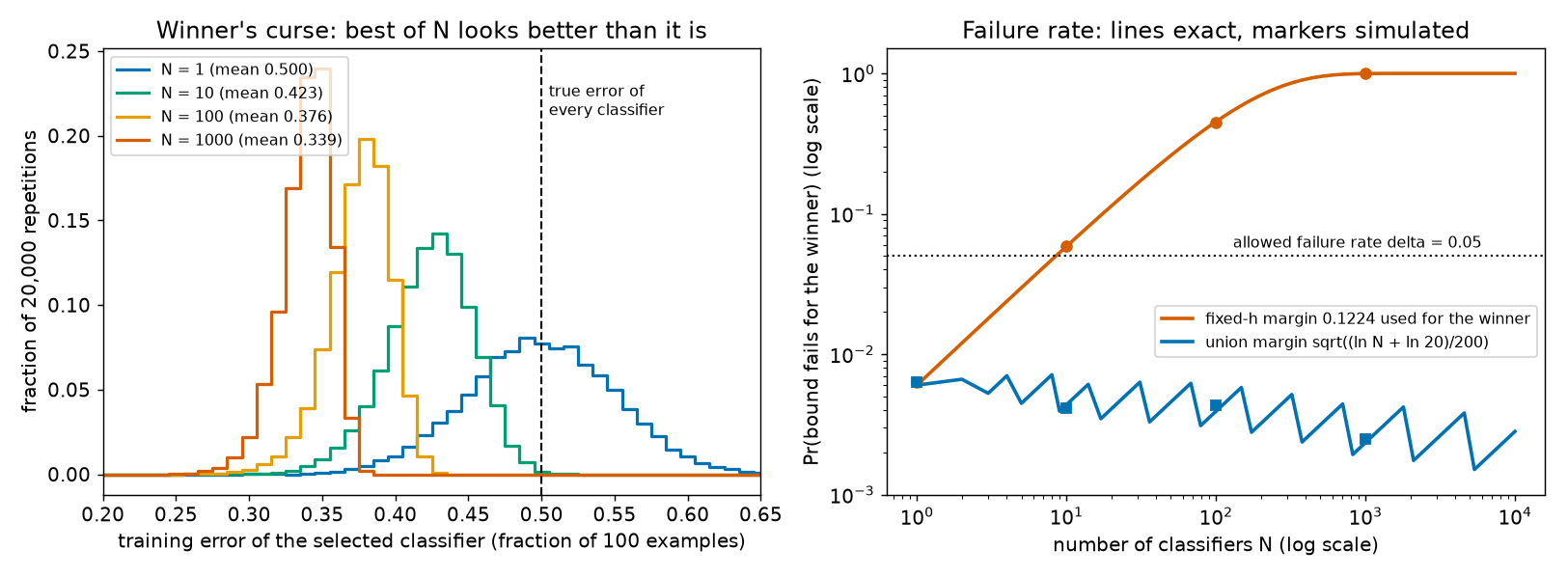
What to notice:
- The winner's curse grows with \(N\). The left panel shifts left as \(N\) grows, although every classifier's true error is 0.5. For \(N = 1000\), the middle 90 % of winners have training errors between 0.31 and 0.36.
- The naive margin breaks quickly. Already at \(N = 10\) it fails in 5.86 % of repetitions (exact), more than the promised 5 %. At \(N = 1000\) it fails almost always.
- The union margin never breaks more than allowed. Its exact failure rate is at most 0.60 % for every \(N\) in the table (the simulated rates differ from it only by simulation noise), far below the allowed 5 %. For \(N = 1000\) the average certificate is \(0.3392 + 0.2225 = 0.5617\), above the true 0.5.
- The sawtooth in the blue curve appears because a training error can only be a whole number of mistakes out of
- The bound fails when the winner makes at most 37 mistakes (naive margin) or at most 27 (union margin, \(N = 1000\)).
The "exact" columns come from a formula derived in a deeper block below. Section [3] of the script repeats the \(N = 1000\) case with explicit coin-flip predictions instead of the formula's shortcut: mean winner error 0.3399 against the exact 0.3393.
(b) Where the slack is¶
Why does the union margin fail in only 0.23 % of repetitions when 5 % was allowed? Section [4] of the script splits the answer into its two steps, for \(N = 1000\) and the union margin 0.2225.
- Hoeffding's step is loose. One classifier fails with probability \(2.346\times 10^{-6}\). Hoeffding allowed \(5.000\times 10^{-5}\), far more (Chapter 9 explains why: it ignores the exact shape of the distribution).
- The union step is almost exact here. Summing over 1,000 classifiers gives 0.0023. The exact probability that some classifier fails is also 0.0023. These bad events are independent and rare, so they hardly overlap.
For the naive margin the same split is instructive. One classifier fails with probability \(6.016\times 10^{-3}\). The sum over 1,000 is 6.0165, a "probability" above 1, so the union bound says nothing; the exact probability is 0.9976.
(c) Near-copies: the union bound overcharges¶
Section [5] replaces the 1,000 independent classifiers with 1,000 near-copies of one classifier, each disagreeing with it on 2 % of inputs. Their true errors are still exactly 0.5.
- The winner's mean training error is 0.4508, against 0.3392 for independent classifiers. Choosing among near-copies is barely a choice.
- The naive margin fails in 5.42 % of repetitions: almost within its promise.
- The union margin for \(N = 1000\) fails in 0.01 % of repetitions: it paid for 1,000 independent choices that did not exist.
The union bound cannot see that hypotheses resemble each other. Its charge depends only on how many there are.
(d) GPT-2 small, counted¶
PAPER §A.1, Note, p. 13 The paper argues that float32 networks form a finite class.
MY EXPLANATION Let us take the argument literally and apply the Occam bound. GPT-2 small is the smallest model of the GPT-2 family of language models and the paper's main architecture (Chapter 5 builds it). In nanoGPT's counting convention (nanoGPT is the open-source GPT-2 code the paper builds on; Chapter 5 again) it has \(D = 123{,}689{,}472\) parameters. Then (script section [6]):
- \(\log_2\lvert\mathcal H\rvert = 32D = 3{,}958{,}063{,}104\) bits;
- \(\ln\lvert\mathcal H\rvert = 32D\ln 2 = 2.7435\times 10^{9}\) nats.
Use \(m = 8{,}009{,}762\) documents [SOURCE: nanoGPT prepare.py split; authors' code default num_docs; erratum
E32] and \(\delta = 0.05\) [SOURCE: authors' code epsilon=0.05; erratum E31].
- For a loss in \([0,1]\) (\(\Delta = 1\)), such as the 0-1 loss or the paper's top-1 error (the fraction of tokens whose most likely prediction is wrong; Chapter 6), the gap term is 13.0867. An error rate is never above 1, so a bound of "training error plus 13" is vacuous in every sense.
- For bits per token (the model's average surprise per token, in bits; Chapter 6), the paper first caps the loss by prediction smoothing, mixing the model's prediction with a uniform guess (Chapter 16). With mixing weight 0.1 the loss lies in an interval of width \(\Delta = 18.787\) bits/token. The gap term is 245.86 bits/token, against 15.617 bits/token for random guessing.
How far off is this? With \(\Delta = 1\), a gap of 0.1 would need \(1.372\times 10^{11}\) documents, 17,126 times the size of OpenWebText. Turned around: at \(m = 8{,}009{,}762\), a gap of 0.1 allows at most \(\ln\lvert\mathcal H\rvert = 160{,}192.2\) nats, that is 231,109 bits, enough to name a model of 7,222 float32 numbers.
Storing the weights more coarsely does not rescue counting. At 16 bits per parameter the gap term is 9.2537; even at 1 bit per parameter it is 2.3134. Counting every network of GPT-2's size is far too expensive. The paper's way out is to weight hypotheses by how short a description they have, so that a model with a short description pays little even inside an enormous class (Chapter 11, Chapter 14).
(e) The same issue inside the paper's pipeline¶
Paper erratum E07: a choice made on the subsample without a union over the candidates
PAPER §6.1, p. 6; App. C, p. 15 Later, the paper estimates the training error on a random subsample of \(n = 10{,}000\) documents (Chapter 17) and keeps, among several settings, the one with the best bound on that subsample. The extra Hoeffding term for the subsample, \(\Delta\sqrt{\ln(1/((1-s)\delta))/(2n)}\) with \(s = n/(n+m)\), is the margin for one fixed hypothesis.
MY EXPLANATION This is the situation of this chapter: a winner chosen on the same data that certifies it. A union over the \(N_{\text{sel}}\) compared candidates replaces \(\ln\frac{1}{(1-s)\delta}\) by \(\ln\frac{N_{\text{sel}}}{(1-s)\delta}\). With \(N_{\text{sel}} = 576\), the whole hyperparameter grid (erratum E07), script section [7] gives: for \(\Delta = 1\) the term grows from 0.0122 to 0.0216 (+0.0094); for \(\Delta = 18.787\) bits/token it grows from 0.2300 to 0.4063 (+0.1763 bits/token). Small, but the published bounds are not covered by the theorem as written (erratum E07).
Going deeper¶
Everything in this section is MY EXPLANATION unless tagged.
The five blocks below prove the union bound, prove the winner's curse inequality and the exact formulas used in the demo, derive the Occam bound step by step, measure how loose the union bound can be, and explain what happens when the class is infinite.
Going deeper: proof of the union bound
Statement. For events \(E_1, E_2, \dots\) (a finite list \(E_1, \dots, E_N\) or an endless list), \(\Pr[\bigcup_i E_i] \le \sum_i \Pr[E_i]\).
Tools from Chapter 1. Additivity: for disjoint events \(F_1, F_2, \dots\), \(\Pr[\bigcup_i F_i] = \sum_i \Pr[F_i]\) (axiom 3, which allows endless lists). Monotonicity: if \(F \subseteq E\) then \(\Pr[F] \le \Pr[E]\).
Step 1: make the events disjoint. Define
\(F_i\) contains the outcomes that lie in \(E_i\) but in none of the earlier events. Think of it as "\(E_i\) is the first event that happens".
Step 2: three facts about the \(F_i\).
- (i) \(F_i \subseteq E_i\), by definition.
- (ii) The \(F_i\) are disjoint. Take \(i < j\). An outcome in \(F_j\) lies in none of \(E_1, \dots, E_{j-1}\), so in particular not in \(E_i\), so not in \(F_i \subseteq E_i\).
- (iii) \(\bigcup_i F_i = \bigcup_i E_i\). By (i), the left side is inside the right side. Conversely, take an outcome \(\omega\) in some \(E_i\), and let \(k\) be the smallest index with \(\omega \in E_k\) (it exists, because every non-empty set of positive whole numbers has a smallest element). Then \(\omega\) is in \(E_k\) and in none of \(E_1, \dots, E_{k-1}\), so \(\omega \in F_k\).
Step 3: add up.
The first equality is fact (iii). The second is additivity, allowed by fact (ii). The inequality applies monotonicity to each term, using fact (i). For an endless list, the sums are endless sums of non-negative terms; the inequality between them holds term by term, so it holds for the totals (which may be \(+\infty\)). \(\square\)
A second proof, with indicators (finite lists). For every outcome, \(\mathbf 1[\bigcup_i E_i] \le \sum_i \mathbf 1[E_i]\): if no event happens both sides are 0; if \(k \ge 1\) events happen the left side is 1 and the right side is \(k\). Take expectations; by monotonicity and linearity, and since the expectation of an indicator is the probability of its event, the union bound follows.
When is it exact? The only inequality used is \(\Pr[F_i] \le \Pr[E_i]\), which is an equality when \(\Pr[E_i \setminus F_i] = 0\), that is, when \(E_i\) overlaps the earlier events only on outcomes of probability 0. So the union bound is exact for disjoint events and loose for overlapping ones.
When is it useless? If \(\sum_i \Pr[E_i] \ge 1\) the statement is true but says nothing. The naive margin in worked example (b) produced a sum of 6.0165.
Complement form, as used for bounds. By the complement rule, \(\Pr[\text{no } E_i \text{ happens}] = 1 - \Pr[\bigcup_i E_i] \ge 1 - \sum_i \Pr[E_i]\).
Going deeper: the winner's curse, proved, and the exact formulas behind the demo
Winner's curse for empirical risk minimization. Let \(\hat h\) be any hypothesis with the smallest empirical risk on the training set. Fix any \(h \in \mathcal H\) (chosen before the data). Then, for every training set, \(\hat R(\hat h) \le \hat R(h)\). Take expectations over the training set (monotonicity): \(\mathbb E[\hat R(\hat h)] \le \mathbb E[\hat R(h)] = R(h)\). The last equality holds because \(h\) is fixed (Chapter 2). Since \(h\) was arbitrary, \(\mathbb E[\hat R(\hat h)] \le \min_h R(h)\).
For the right half: for every training set, \(R(\hat h) \ge \min_h R(h)\), because \(\hat h\) is one member of the class. Taking expectations gives \(\mathbb E[R(\hat h)] \ge \min_h R(h)\). Together:
Random: the training set, hence \(\hat h\), \(\hat R(\hat h)\) and \(R(\hat h)\). Fixed: \(\mathcal H\) and every \(R(h)\). The expectations are over the training set. A finite class guarantees that a minimizer exists.
The simulation model. Labels are fair coins independent of the input, so for any fixed classifier the mistake indicator \(\mathbf 1[h(z) \ne y]\) is a fair coin: true error exactly 0.5. The \(N\) classifiers are lookup tables of fair-coin guesses, drawn before the data. On \(m\) distinct training inputs, the \(N \times m\) mistake indicators are then independent fair coins (each is a guess compared with an independent fair coin). So each classifier's mistake count \(K_i\) is Binomial\((m, \tfrac12)\), independently across classifiers. The script draws these counts directly; section [3] checks the shortcut against explicit coin flips.
Exact failure probability. Write \(F(k) = \Pr[K_i \le k]\) for the Binomial\((100, \tfrac12)\) distribution function. The certificate "true error \(<\) training error \(+\,t\)" fails for the winner exactly when \(0.5 \ge K_{\min}/100 + t\), that is, when \(K_{\min} \le k_t = \lfloor 100(0.5 - t)\rfloor\), where \(K_{\min} = \min_i K_i\). By independence,
With \(t = 0.1224\), \(k_t = 37\); with \(t = 0.2225\), \(k_t = 27\).
Exact mean of the winner's training error. For a random whole number \(K \ge 0\), \(K = \sum_{k \ge 0}\mathbf 1[K > k]\) (the right side counts the numbers \(0, 1, \dots, K-1\)). Taking expectations, \(\mathbb E[K] = \sum_{k\ge0}\Pr[K > k]\). Applied to \(K_{\min} \le 100\):
which gives 0.3393 for \(N = 1000\).
Why the losses of the winner are not independent. The winner's loss on example \(j\) depends on which classifier won, and that depends on all 100 examples. Knowing that the winner erred on examples 1 to 50 makes it less likely that it also erred on example 51, because a classifier with so many mistakes would rarely have won. This is the failure of step (c) in Chapter 9's proof.
Going deeper: the Occam bound, derived step by step
Setting. \(\mathcal H\) is a finite list of \(N\) hypotheses, fixed before the data. For each \(h\), the losses \(R(h, X_1), \dots, R(h, X_m)\) lie in an interval \([a, a+\Delta]\) fixed in advance (loss units), and the documents \(X_j\) are i.i.d.
Step 1 (one fixed hypothesis). For a fixed \(h\) the losses are independent, with mean \(R(h)\). Chapter 9's lower-tail Hoeffding inequality gives, for every \(t > 0\),
The probability is over the documents; \(h\), \(R(h)\), \(t\), \(m\) and \(\Delta\) are fixed.
Step 2 (choose the margin). Solve \(\exp(-2mt^2/\Delta^2) = \delta/N\). Take \(\ln\) of both sides: \(-2mt^2/\Delta^2 = \ln(\delta/N) = -\ln(N/\delta)\). Multiply by \(-\Delta^2/(2m)\): \(t^2 = \Delta^2\ln(N/\delta)/(2m)\). Take the positive square root and use \(\ln(N/\delta) = \ln N + \ln(1/\delta)\):
Units: \(\ln N\) and \(\ln(1/\delta)\) are pure numbers (nats), \(m\) is a count, so \(t_N\) has the units of \(\Delta\).
Step 3 (union). With \(E_h = \{R(h) \ge \hat R(h) + t_N\}\), the union bound and Step 1 give \(\Pr[\bigcup_h E_h] \le \sum_h \Pr[E_h] \le N \cdot \delta/N = \delta\).
Step 4 (complement). With probability at least \(1-\delta\), no \(E_h\) happens: \(R(h) < \hat R(h) + t_N\) for all \(h \in \mathcal H\) at once.
Step 5 (the trained hypothesis). \(\hat h \in \mathcal H\), so on the same event \(R(\hat h) < \hat R(\hat h) + t_N\). \(\square\)
Two-sided version. To bound \(\lvert R(h) - \hat R(h)\rvert\), use both tails: \(2N\) events, each with share \(\delta/(2N)\), giving the margin \(\Delta\sqrt{\ln(2N/\delta)/(2m)}\).
How much data. To make the margin at most \(\varepsilon\), square and solve: \(m \ge \Delta^2(\ln N + \ln(1/\delta))/(2\varepsilon^2)\). The data needed grows only with \(\ln N\). For float32 GPT-2 small with \(\Delta = 1\) and \(\varepsilon = 0.1\) this gives the \(1.372\times 10^{11}\) documents of worked example (d).
Check against the paper's form. Eq. (1) has \(\ln(1/P(h))\) where we have \(\ln N\). With \(P(h) = 1/N\) for every \(h\), the two agree. The script computes the GPT-2 numbers by calling the shared Eq. (1) function with \(\ln(1/P(h)) = \ln\lvert\mathcal H\rvert\).
Going deeper: how loose is the union bound?
A matching lower bound. For events \(E_1, \dots, E_N\),
Proof with indicators. Fix an outcome and let \(k\) be the number of events it lies in. The left indicator is 1 if \(k \ge 1\) and 0 if \(k = 0\). The right side counts \(k - k(k-1)/2\), since \(\sum_{i<j}\mathbf 1[E_i]\mathbf 1[E_j]\) counts pairs of events that both happen. Check every \(k\): \(k = 0\) gives \(0 \ge 0\); \(k = 1\) gives \(1 \ge 1\); \(k = 2\) gives \(1 \ge 1\); \(k \ge 3\) gives \(k(3-k)/2 \le 0 < 1\). So the inequality holds outcome by outcome; take expectations. \(\square\)
Consequence. The union bound overstates the true probability by at most the total pairwise overlap \(\sum_{i<j}\Pr[E_i \cap E_j]\). For independent rare events the overlaps are products of small numbers, so the bound is nearly exact: in worked example (b), sum 0.0023 against exact 0.0023. For near-copies the overlaps are almost as large as the events themselves, and the bound can overstate by a factor close to \(N\): in worked example (c), the 1,000 near-copies behave almost like a single hypothesis.
What this means for learning. All hypotheses are evaluated on the same documents, so hypotheses that predict similarly have overlapping bad events. Counting cannot exploit this. Classical theory has tools that do (they measure how many genuinely different labelings a class can produce on the data; Chapter 23 surveys them). The paper instead keeps the union bound and changes the shares (Chapter 11).
Going deeper: infinite classes, and what must be fixed in advance
Countably infinite classes. The union bound holds for endless lists, so the argument still works if every hypothesis gets a share \(\delta_h > 0\) with \(\sum_h \delta_h \le \delta\). Equal shares are impossible: they would be \(\delta/\infty = 0\), and a share of 0 needs an infinite margin. The shares must therefore be unequal, for example \(\delta_h = \delta\,2^{-k}\) for the \(k\)-th hypothesis in a fixed list (\(k = 1, 2, \dots\)), which adds up to \(\delta\). Unequal shares fixed in advance are exactly a prior; Chapter 11 develops this.
Uncountable classes. If parameters are true real numbers, there are uncountably many hypotheses. A sum of uncountably many positive numbers is infinite, so the union bound cannot be used directly. PAPER §A.1, Note, p. 13 The paper sidesteps this by observing that stored weights have finite precision. MY EXPLANATION That observation is correct, and it is all the union bound needs.
Overcounting is harmless. Different bit patterns can give the same network (for example \(+0\) and \(-0\), or the many patterns that mean "not a number"), so \(2^{32D}\) overstates the number of distinct hypotheses. Overstating a count only loosens the bound.
Everything chosen with the data belongs to the hypothesis. The architecture, the hyperparameters and any selection among runs must either be fixed before the data or be counted as part of \(h\) (Chapter 2 defined a hypothesis to include hyperparameters). If they were chosen by looking at the data, the class must include every option that could have been chosen. The paper pays for its hyperparameter choices in its complexity term (Chapter 24); erratum E07 (above) concerns a choice whose price is missing from one term.
Common misconceptions¶
Everything in this section is MY EXPLANATION.
- Misconception: The union bound needs the events to be independent. — Actually: it holds for any events whatsoever. Independence matters only for how tight it is: nearly exact for independent rare events (0.0023 versus 0.0023 in worked example (b)), very loose for overlapping ones (worked example (c)).
- Misconception: If the bound holds with probability 95 % for each hypothesis, it holds with probability 95 % for the one training picks. — Actually: each of 1,000 classifiers failed its naive bound with probability only 0.0060, yet the winner's naive bound failed with probability 0.9976. A guarantee for the winner needs a simultaneous guarantee for all hypotheses.
- Misconception: Only the hypotheses that training actually tried need to be counted. — Actually: the count must cover every hypothesis that training could have returned, for any training set, and it must be fixed before the data. Which hypotheses gradient descent visits depends on the data, so the visited ones are not a valid class.
- Misconception: A bigger hypothesis class makes the bound much worse. — Actually: the price grows like \(\ln\lvert\mathcal H\rvert\): 1,000 times more hypotheses adds 6.9078 nats. And once hypotheses are weighted instead of counted (Chapter 11), the size of the class no longer matters by itself.
- Misconception: The vacuous counting bound for GPT-2 (gap term 13.0867) shows that GPT-2 does not generalize. — Actually: a vacuous bound says nothing either way. It shows that counting is the wrong way to measure a large model's complexity.
- Misconception: Storing weights in fewer bits would make counting work. — Actually: even at 1 bit per parameter the gap term is 2.3134, still vacuous for a loss in \([0,1]\). The number of trainable values must shrink drastically, which is what the paper's compression does.
Self-test¶
Q1. A team fixes 64 candidate models before seeing any data, then evaluates all of them on \(m = 10{,}000\) documents with a loss in \([0,1]\), and reports the best one. With \(\delta = 0.05\), what margin does the Occam bound add to the winner's empirical risk? Compare it with the margin for a single model fixed in advance.
Answer
Single model: \(\sqrt{\ln 20/(2\times 10{,}000)} = 0.012239\). Winner of 64: \(\sqrt{(\ln 64 + \ln 20)/20{,}000} = 0.018914\), where \(\ln 64 = 4.1589\) nats \(= 6\) bits \(\times \ln 2\) (script section [8]). Choosing among 64 candidates costs 6 bits, and raises the margin from 0.012239 to 0.018914.
Q2. In the demo with \(N = 1000\), the statement "with probability at least 0.95, every classifier satisfies \(R(h) < \hat R(h) + 0.2225\)" is true. What is random and what is fixed in it? Why does the statement then also cover the winner? And what goes wrong if, after looking at the data, you keep only the 10 classifiers with the lowest training error and use the margin for \(N = 10\)?
Answer
Random: the 100 training examples, hence every \(\hat R(h)\), the winner \(\hat h\) and its \(\hat R(\hat h)\). Fixed: the 1,000 classifiers (drawn before the data), their true errors (0.5 each), \(m\), \(\delta\) and the margin 0.2225. The "0.95" is over repeated draws of the training set.
The statement asserts one event on which all 1,000 inequalities hold together. The winner is one of the 1,000, so on that event its inequality holds too, however it was chosen.
Keeping "the 10 best" is a choice made with the data. The 10-member list is itself random, so the union over 10 fixed hypotheses does not apply. The real amount of choice was among 1,000 classifiers, and the margin must be the one for \(N = 1000\).
Q3. Redo the GPT-2 small counting bound (loss in \([0,1]\), \(m = 8{,}009{,}762\) SOURCE: nanoGPT, \(\delta = 0.05\) SOURCE: authors' code) with weights stored in 16 bits instead of 32, and then with 1 bit per parameter. Is either bound non-vacuous?
Answer
The count becomes \(\lvert\mathcal H\rvert \le 2^{bD}\) with \(b\) bits per parameter, so \(\ln\lvert\mathcal H\rvert = bD\ln 2\) and the gap term is \(\sqrt{(bD\ln 2 + \ln 20)/(2m)}\). The script gives 9.2537 for \(b = 16\) and 2.3134 for \(b = 1\) (section [6]). Both exceed 1, so both are vacuous: an error rate is never above 1. Halving the bits only divides the gap term by about \(\sqrt 2\). A non-vacuous bound needs far fewer free values, not slightly cheaper ones; at OpenWebText's size a gap of 0.1 allows about 231,109 bits in total.
Code for this chapter¶
Run it from the project root:
.venv/Scripts/python explainer/code/ch10_union.py
Source: ch10_union.py
"""Chapter 10 demo: the winner's curse and the union-bound repair.

Claims reproduced / illustrated
  * Selection bias (winner's curse): among N classifiers whose true error is exactly 0.5,
    the one with the lowest training error on m = 100 examples looks much better than 0.5.
  * A Hoeffding margin for ONE fixed hypothesis, sqrt(ln(1/delta)/(2m)), applied to the
    selected winner fails far more often than delta (paper App. A.1, p. 13: h* (our h_hat) "was
    constructed using the training data").
  * The union bound Pr(E_1 or ... or E_N) <= sum_i Pr(E_i) repairs it: the margin
    sqrt((ln N + ln(1/delta))/(2m)) holds for all N hypotheses at once, hence for the winner
    (the Occam bound for a finite class; paper App. A.1 with a uniform prior P(h) = 1/N).
  * The union bound is pessimistic when the hypotheses are near-duplicates.
  * The paper's Note (App. A.1, p. 13): float32 networks form a finite class. Counting
    |H| = 2^(32 D) for GPT-2 small (D = 123,689,472, nanoGPT count via pacbound.gpt2_params)
    with m = 8,009,762 [SOURCE nanoGPT / authors' code] and delta = 0.05 [SOURCE authors'
    code] gives a gap term of about 13 for a loss in [0, 1]: vacuous.
  * Erratum E07 arithmetic: the n-term of Eq. (3) with and without a union over 576 candidates.

Simulation model (sections [2], [5]). Labels are pure noise: each label is a fair coin,
independent of the input, so EVERY fixed classifier has true 0-1 error exactly 0.5. Each
classifier is a lookup table of fair-coin guesses drawn before the data. With distinct
training inputs, the N x m mistake indicators are then i.i.d. Bernoulli(0.5), so each
classifier's number of training mistakes is Binomial(m, 0.5), independently across
classifiers. The script draws these counts directly; section [3] checks the shortcut against
explicit coin-flip predictions.

Outputs: code/outputs/ch10_union.txt, docs/assets/fig/ch10_winners_curse.png
"""
from __future__ import annotations

import math
import sys
import time
from pathlib import Path

import numpy as np
from scipy.stats import binom

import matplotlib
matplotlib.use("Agg")
import matplotlib.pyplot as plt

HERE = Path(__file__).resolve().parent
sys.path.insert(0, str(HERE))
import pacbound as pb  # noqa: E402

OUT_TXT = HERE / "outputs" / "ch10_union.txt"
FIG_DIR = HERE.parent / "docs" / "assets" / "fig"
FIG = FIG_DIR / "ch10_winners_curse.png"

M = 100                    # training examples in the toy experiment
DELTA = pb.DELTA           # 0.05 [SOURCE authors' code]
NS = [1, 10, 100, 1000]    # numbers of classifiers
REPS = 20_000              # repetitions of the whole experiment
TRUE_ERR = 0.5             # true 0-1 error of every classifier (labels are pure noise)
FLIP = 0.02                # section [5]: a near-copy disagrees with the base on 2 % of inputs

lines: list[str] = []


def out(s: str = "") -> None:
    print(s)
    lines.append(s)


def margin(n_hyp: int, m: int = M, delta: float = DELTA, width: float = 1.0) -> float:
    """Occam margin width*sqrt((ln N + ln 1/delta)/(2m)); N = 1 is the fixed-h Hoeffding margin.
    Uses pacbound.hoeffding_t with ln(N/delta) nats. Loss units."""
    return pb.hoeffding_t(m, width, math.log(n_hyp) + math.log(1.0 / delta))


def k_fail(t: float, m: int = M) -> int:
    """Largest mistake count K with K/m <= TRUE_ERR - t, i.e. the bound 'R < Rhat + t' fails.
    Returns -1 if no count fails."""
    return math.floor(m * (TRUE_ERR - t) + 1e-12)


def p_fail_exact(n_hyp: int, t: float, m: int = M) -> float:
    """Exact Pr(winner's bound fails) = Pr(min of N Binomial(m,1/2) counts <= k_fail)."""
    k = k_fail(t, m)
    if k < 0:
        return 0.0
    f = binom.cdf(k, m, 0.5)
    return -math.expm1(n_hyp * math.log1p(-f))          # 1 - (1 - f)^N, computed stably


def mean_min_exact(n_hyp: int, m: int = M) -> float:
    """E[min of N Binomial(m,1/2)]/m via E[min] = sum_{k=0}^{m-1} Pr(min > k) = sum (1-F(k))^N."""
    ks = np.arange(m)
    surv = (1.0 - binom.cdf(ks, m, 0.5)) ** n_hyp
    return float(surv.sum()) / m


def main() -> None:
    t0 = time.time()
    rng = np.random.default_rng(0)
    OUT_TXT.parent.mkdir(parents=True, exist_ok=True)
    FIG_DIR.mkdir(parents=True, exist_ok=True)

    out("Chapter 10 - the union bound  (ch10_union.py)")
    out("=" * 60)

    # [A] analogy: multiple comparisons -----------------------------------------
    k_tests, a = 20, 0.05
    out(f"[A] {k_tests} independent tests at false-alarm rate {a}: Pr(>= 1 false alarm) = "
        f"{1 - (1 - a) ** k_tests:.4f}")
    out(f"    Bonferroni: each at {a / k_tests:.4f}; union bound {k_tests * (a / k_tests):.4f}; "
        f"exact {1 - (1 - a / k_tests) ** k_tests:.4f}")
    out()

    # [1] margins -------------------------------------------------------------
    out("[1] Margins for m = 100 examples, 0-1 loss (Delta = 1), delta = 0.05")
    t1 = margin(1)
    out(f"  ln(1/delta) = ln 20 = {math.log(20):.6f} nats")
    out(f"  fixed-h Hoeffding margin sqrt(ln20/200)        = {t1:.6f}")
    for n in NS[1:]:
        out(f"  union margin N = {n:>4}: sqrt((ln {n:<4} + ln 20)/200) = {margin(n):.6f}"
            f"   (ln N = {math.log(n):.4f} nats)")
    # Hoeffding * N at the union margin must equal delta exactly
    for n in NS:
        tot = n * pb.hoeffding_tail(margin(n), M, 1.0)
        assert abs(tot - DELTA) < 1e-12, tot

    # [2] best-of-N simulation --------------------------------------------------
    out()
    out(f"[2] Best of N coin-flip classifiers, true error 0.5 each, {REPS:,} repetitions")
    out(f"  bound fails when the winner's mistakes K <= {k_fail(t1)} (naive margin) or "
        f"<= {k_fail(margin(1000))} (union margin, N = 1000)")
    out("    N  mean winner err (sim/exact)  naive fail (sim/exact)  union fail (sim/exact)")
    winners: dict[int, np.ndarray] = {}
    for n in NS:
        counts = rng.binomial(M, 0.5, size=(REPS, n))
        kmin = counts.min(axis=1)
        winners[n] = kmin / M
        mean_sim = winners[n].mean()
        mean_ex = mean_min_exact(n)
        naive_sim = float(np.mean(kmin <= k_fail(t1)))
        naive_ex = p_fail_exact(n, t1)
        tn = margin(n)
        uni_sim = float(np.mean(kmin <= k_fail(tn)))
        uni_ex = p_fail_exact(n, tn)
        out(f"  {n:>4}      {mean_sim:.4f} / {mean_ex:.4f}         "
            f"{naive_sim:.4f} / {naive_ex:.4f}         {uni_sim:.4f} / {uni_ex:.4f}")
        se = math.sqrt(0.25 / (M * REPS))           # generous SE for the mean
        assert abs(mean_sim - mean_ex) < 6 * se + 1e-3
        for sim, ex in ((naive_sim, naive_ex), (uni_sim, uni_ex)):
            assert abs(sim - ex) < 5 * math.sqrt(max(ex * (1 - ex), 1e-6) / REPS) + 1e-4
        assert uni_ex <= DELTA and uni_sim <= DELTA
    w1000 = winners[1000]
    q05, q50, q95 = np.quantile(w1000, [0.05, 0.5, 0.95])
    out(f"  N = 1000: winner's training error 5/50/95 % quantiles = {q05:.2f} / {q50:.2f} / {q95:.2f}")
    out(f"  N = 1000: mean winner err + naive margin = {w1000.mean() + t1:.4f}  (< 0.5: wrong 'certificate')")
    out(f"  N = 1000: mean winner err + union margin = {w1000.mean() + margin(1000):.4f}  (> 0.5: covers)")
    out(f"  N = 1000: mean selection gap R(h_hat) - Rhat(h_hat) = {TRUE_ERR - w1000.mean():.4f}")
    assert p_fail_exact(1000, t1) > 0.99

    # [3] explicit check of the binomial shortcut -------------------------------
    reps_x, chunk = 2_000, 100
    mins = []
    for _ in range(reps_x // chunk):
        labels = rng.integers(0, 2, size=(chunk, 1, M), dtype=np.int8)
        preds = rng.integers(0, 2, size=(chunk, 1000, M), dtype=np.int8)
        mins.append((preds != labels).sum(axis=2).min(axis=1))
    mean_x = np.concatenate(mins).mean() / M
    out()
    out(f"[3] Explicit coin-flip predictions vs labels ({reps_x:,} reps, N = 1000): "
        f"mean winner err = {mean_x:.4f} (exact {mean_min_exact(1000):.4f})")
    assert abs(mean_x - mean_min_exact(1000)) < 0.003

    # [4] where the looseness sits, N = 1000 ------------------------------------
    out()
    out("[4] Union bound vs exact, N = 1000 independent classifiers")
    for name, t in (("naive margin", t1), ("union margin", margin(1000))):
        p1 = binom.cdf(k_fail(t), M, 0.5)
        out(f"  {name} {t:.4f}: one classifier fails w.p. {p1:.3e} (Hoeffding says <= "
            f"{pb.hoeffding_tail(t, M, 1.0):.3e})")
        out(f"      sum over 1000 = {1000 * p1:.4f};  exact Pr(some classifier fails) = "
            f"{p_fail_exact(1000, t):.4f}")

    # [5] near-duplicate classifiers ------------------------------------------
    out()
    out(f"[5] N = 1000 near-copies of one classifier (each disagrees on {FLIP:.0%} of inputs)")
    k0 = rng.binomial(M, 0.5, size=(REPS, 1))                  # base classifier's mistakes
    ki = k0 - rng.binomial(np.broadcast_to(k0, (REPS, 1000)), FLIP) \
        + rng.binomial(np.broadcast_to(M - k0, (REPS, 1000)), FLIP)
    kmin_dup = ki.min(axis=1)
    out(f"  mean winner err = {kmin_dup.mean() / M:.4f}  (independent classifiers: "
        f"{winners[1000].mean():.4f})")
    out(f"  naive margin fails in {np.mean(kmin_dup <= k_fail(t1)):.4f} of reps; "
        f"union margin (N = 1000) fails in {np.mean(kmin_dup <= k_fail(margin(1000))):.4f}")

    # [6] counting float32 GPT-2 small ----------------------------------------
    out()
    out("[6] Counting hypotheses: GPT-2 small stored as float32 (paper's Note, App. A.1)")
    D = pb.gpt2_params(12, 768)
    assert D == 123_689_472
    m_docs = pb.M_DOCS
    bits = 32 * D
    ln_h = pb.bits_to_nats(bits)
    gap1 = pb.eq1_complexity(ln_h, m_docs, DELTA, 1.0)
    _, _, w_bpd = pb.smoothing_interval(0.1)
    gap_bpd = pb.eq1_complexity(ln_h, m_docs, DELTA, w_bpd)
    out(f"  D = {D:,} parameters (nanoGPT count); log2|H| = 32 D = {bits:,} bits")
    out(f"  ln|H| = 32 D ln 2 = {ln_h:.4e} nats;  m = {m_docs:,} [SOURCE]; delta = 0.05 [SOURCE]")
    out(f"  (ln 2 = {pb.LN2:.6f} nats per bit; 1/ln 2 = {1 / pb.LN2:.6f})")
    out(f"  gap term, loss in [0,1] (Delta = 1)            = {gap1:.4f}   (any error is <= 1)")
    out(f"  gap term, Delta = {w_bpd:.3f} bits/token (alpha = 0.1) = {gap_bpd:.2f} bits/token"
        f"   (random guess {pb.random_guess_bpd():.3f})")
    assert 13.0 < gap1 < 13.2
    target = 0.1
    m_need = (ln_h + math.log(1 / DELTA)) / (2 * target ** 2)
    out(f"  documents needed for a gap of {target} (Delta = 1): {m_need:.3e}"
        f" = {m_need / m_docs:,.0f} x OpenWebText")
    ln_max = 2 * m_docs * target ** 2 - math.log(1 / DELTA)
    out(f"  at m = {m_docs:,}, gap <= {target} allows ln|H| <= {ln_max:,.1f} nats"
        f" = {pb.nats_to_bits(ln_max):,.0f} bits = {pb.nats_to_bits(ln_max) / 32:,.0f} float32 numbers")
    for b in (16, 1):
        g = pb.eq1_complexity(pb.bits_to_nats(b * D), m_docs, DELTA, 1.0)
        out(f"  {b:>2} bit(s) per parameter: gap term (Delta = 1) = {g:.4f}")

    # [7] erratum E07: union over candidates compared on the subsample -----------
    out()
    out("[7] Erratum E07: n-term of Eq. (3), n = 10,000, s = n/(n+m), without / with a union over 576")
    for w, unit in ((1.0, "(fraction)"), (w_bpd, "bits/token")):
        _, a = pb.eq3_terms(0.0, m_docs, pb.N_SUB, DELTA, w, n_selected=1)
        _, b = pb.eq3_terms(0.0, m_docs, pb.N_SUB, DELTA, w, n_selected=576)
        out(f"  Delta = {w:.3f}: {a:.4f} -> {b:.4f}  (+{b - a:.4f} {unit})")

    # [8] self-test numbers ---------------------------------------------------
    out()
    out("[8] Self-test: N = 64 candidates fixed in advance, m = 10,000, Delta = 1, delta = 0.05")
    out(f"  one fixed model: {margin(1, 10_000):.6f};  winner of 64: {margin(64, 10_000):.6f}"
        f"  (ln 64 = {math.log(64):.4f} nats = 6 bits)")

    # figure ------------------------------------------------------------------
    plt.rcParams.update({"font.size": 11})
    fig, (ax1, ax2) = plt.subplots(1, 2, figsize=(12.5, 4.6))
    colors = {1: "#0072B2", 10: "#009E73", 100: "#E69F00", 1000: "#D55E00"}
    grid = np.arange(0, M + 1) / M
    for n in NS:
        vals, cnt = np.unique(np.round(winners[n] * M).astype(int), return_counts=True)
        freq = np.zeros(M + 1)
        freq[vals] = cnt / REPS
        ax1.step(grid, freq, where="mid", color=colors[n], lw=1.8,
                 label=f"N = {n} (mean {winners[n].mean():.3f})")
    ax1.axvline(TRUE_ERR, color="black", ls="--", lw=1.2)
    ax1.text(TRUE_ERR + 0.005, ax1.get_ylim()[1] * 0.92, "true error of\nevery classifier",
             fontsize=9, va="top")
    ax1.set_xlim(0.2, 0.65)
    ax1.set_xlabel("training error of the selected classifier (fraction of 100 examples)")
    ax1.set_ylabel(f"fraction of {REPS:,} repetitions")
    ax1.set_title("Winner's curse: best of N looks better than it is")
    ax1.legend(fontsize=9, loc="upper left")

    n_grid = np.unique(np.round(np.logspace(0, 4, 60)).astype(int))
    naive = [p_fail_exact(int(n), t1) for n in n_grid]
    union = [p_fail_exact(int(n), margin(int(n))) for n in n_grid]
    ax2.plot(n_grid, naive, color="#D55E00", lw=2,
             label="fixed-h margin 0.1224 used for the winner")
    ax2.plot(n_grid, union, color="#0072B2", lw=2,
             label="union margin sqrt((ln N + ln 20)/200)")
    for n in NS:
        ax2.plot(n, np.mean(winners[n] * M <= k_fail(t1)), "o", color="#D55E00", ms=6)
        ax2.plot(n, max(np.mean(winners[n] * M <= k_fail(margin(n))), 1e-4), "s",
                 color="#0072B2", ms=6)
    ax2.axhline(DELTA, color="black", ls=":", lw=1.2)
    ax2.text(130, DELTA * 1.15, "allowed failure rate delta = 0.05", fontsize=9)
    ax2.set_xscale("log")
    ax2.set_yscale("log")
    ax2.set_ylim(1e-3, 1.5)
    ax2.set_xlabel("number of classifiers N (log scale)")
    ax2.set_ylabel("Pr(bound fails for the winner) (log scale)")
    ax2.set_title("Failure rate: lines exact, markers simulated")
    ax2.legend(fontsize=9, loc="lower right", bbox_to_anchor=(1.0, 0.29))
    fig.tight_layout()
    fig.savefig(FIG, dpi=130)
    plt.close(fig)

    out()
    out(f"figure: docs/assets/fig/{FIG.name}")
    print(f"runtime {time.time() - t0:.1f} s (console only, so the output file is deterministic)")
    OUT_TXT.write_text("\n".join(lines) + "\n", encoding="utf-8")


if __name__ == "__main__":
    main()
Output:
Chapter 10 - the union bound  (ch10_union.py)
============================================================
[A] 20 independent tests at false-alarm rate 0.05: Pr(>= 1 false alarm) = 0.6415
    Bonferroni: each at 0.0025; union bound 0.0500; exact 0.0488

[1] Margins for m = 100 examples, 0-1 loss (Delta = 1), delta = 0.05
  ln(1/delta) = ln 20 = 2.995732 nats
  fixed-h Hoeffding margin sqrt(ln20/200)        = 0.122387
  union margin N =   10: sqrt((ln 10   + ln 20)/200) = 0.162762   (ln N = 2.3026 nats)
  union margin N =  100: sqrt((ln 100  + ln 20)/200) = 0.194947   (ln N = 4.6052 nats)
  union margin N = 1000: sqrt((ln 1000 + ln 20)/200) = 0.222525   (ln N = 6.9078 nats)

[2] Best of N coin-flip classifiers, true error 0.5 each, 20,000 repetitions
  bound fails when the winner's mistakes K <= 37 (naive margin) or <= 27 (union margin, N = 1000)
    N  mean winner err (sim/exact)  naive fail (sim/exact)  union fail (sim/exact)
     1      0.4997 / 0.5000         0.0063 / 0.0060         0.0063 / 0.0060
    10      0.4235 / 0.4232         0.0593 / 0.0586         0.0041 / 0.0044
   100      0.3756 / 0.3752         0.4469 / 0.4531         0.0043 / 0.0039
  1000      0.3392 / 0.3393         0.9980 / 0.9976         0.0025 / 0.0023
  N = 1000: winner's training error 5/50/95 % quantiles = 0.31 / 0.34 / 0.36
  N = 1000: mean winner err + naive margin = 0.4616  (< 0.5: wrong 'certificate')
  N = 1000: mean winner err + union margin = 0.5617  (> 0.5: covers)
  N = 1000: mean selection gap R(h_hat) - Rhat(h_hat) = 0.1608

[3] Explicit coin-flip predictions vs labels (2,000 reps, N = 1000): mean winner err = 0.3399 (exact 0.3393)

[4] Union bound vs exact, N = 1000 independent classifiers
  naive margin 0.1224: one classifier fails w.p. 6.016e-03 (Hoeffding says <= 5.000e-02)
      sum over 1000 = 6.0165;  exact Pr(some classifier fails) = 0.9976
  union margin 0.2225: one classifier fails w.p. 2.346e-06 (Hoeffding says <= 5.000e-05)
      sum over 1000 = 0.0023;  exact Pr(some classifier fails) = 0.0023

[5] N = 1000 near-copies of one classifier (each disagrees on 2% of inputs)
  mean winner err = 0.4508  (independent classifiers: 0.3392)
  naive margin fails in 0.0542 of reps; union margin (N = 1000) fails in 0.0001

[6] Counting hypotheses: GPT-2 small stored as float32 (paper's Note, App. A.1)
  D = 123,689,472 parameters (nanoGPT count); log2|H| = 32 D = 3,958,063,104 bits
  ln|H| = 32 D ln 2 = 2.7435e+09 nats;  m = 8,009,762 [SOURCE]; delta = 0.05 [SOURCE]
  (ln 2 = 0.693147 nats per bit; 1/ln 2 = 1.442695)
  gap term, loss in [0,1] (Delta = 1)            = 13.0867   (any error is <= 1)
  gap term, Delta = 18.787 bits/token (alpha = 0.1) = 245.86 bits/token   (random guess 15.617)
  documents needed for a gap of 0.1 (Delta = 1): 1.372e+11 = 17,126 x OpenWebText
  at m = 8,009,762, gap <= 0.1 allows ln|H| <= 160,192.2 nats = 231,109 bits = 7,222 float32 numbers
  16 bit(s) per parameter: gap term (Delta = 1) = 9.2537
   1 bit(s) per parameter: gap term (Delta = 1) = 2.3134

[7] Erratum E07: n-term of Eq. (3), n = 10,000, s = n/(n+m), without / with a union over 576
  Delta = 1.000: 0.0122 -> 0.0216  (+0.0094 (fraction))
  Delta = 18.787: 0.2300 -> 0.4063  (+0.1763 bits/token)

[8] Self-test: N = 64 candidates fixed in advance, m = 10,000, Delta = 1, delta = 0.05
  one fixed model: 0.012239;  winner of 64: 0.018914  (ln 64 = 4.1589 nats = 6 bits)

figure: docs/assets/fig/ch10_winners_curse.png