18. Random subspace training¶
Where this fits
Prerequisites: Chapter 7 (gradient, gradient descent, learning rate, Adam, reparameterization, random initialization, seed, flatten), Chapter 8 (orthonormal columns and \(P^\top P=I\), QR decomposition, Kronecker product, mixed-product property, vec trick, Gaussian random matrix, near-orthogonality). Used later by: Chapter 20 (SubLoRA puts this projector inside LoRA), Chapter 24 (the pipeline and its \(d\) grid), Chapter 28 (the mini replication). Purpose: explain how a network with \(D\) adjustable numbers can be trained by moving only \(d\ll D\) numbers, how the paper builds the matrix that makes this possible, and how good its two recipes are.
The problem this chapter solves¶
MY EXPLANATION GPT-2 small has about 124 million parameters. Written out as 32-bit numbers that is
\(3.958\times10^{9}\) bits (output [7] of ch07_gd.py). Chapter 14 shows that a bound of the paper's kind can only be
non-vacuous if the trained model can be described in far fewer bits, a few hundred thousand at most.
So the model must be trained in a way that leaves very little to describe. One way: let only a short list of \(d\) numbers move during training, and tie all \(D\) parameters to that short list by a fixed rule that is known before training starts. Then the description of the trained model is the short list.
PAPER §3, p. 4 The background section describes exactly this, following Lotfi et al. (2022). All \(D\) weights, flattened into one vector \(\theta\), are written as a random initialization \(\theta_0\) plus a matrix \(P\) (shape \(D\times d\)) times a short vector \(w\) of length \(d\): \(\theta=\theta_0+Pw\). \(P\) is a Kronecker product of two random Gaussian matrices, scaled so that \(P^\top P\approx I\). Only \(w\) is optimized, by backpropagating through this formula. Afterwards \(w\) is quantized and arithmetic-coded (Chapters 21 and 22).
PAPER §5, p. 6 The paper's own method uses a different \(P\): the Kronecker product of two matrices obtained by QR-orthogonalizing Gaussian matrices. PAPER App. E, p. 16 The grid of \(d\) values is \(\{5{,}000;\,10{,}000;\,25{,}000;\,50{,}000;\,100{,}000;\,200{,}000\}\). PAPER Tables 1–2, pp. 6–7 A "Subspace Only" column reports models trained with \(\theta=\theta_0+Pw\) and no LoRA.
MY EXPLANATION This chapter answers six questions:
- Why should training only \(d\) numbers work at all? (Intrinsic dimension.)
- How do gradients reach \(w\)?
- What does \(P^\top P\approx I\) buy, and how close to \(I\) is the §3 recipe really?
- Why is the §5 recipe exact, and what does it cost to store and use?
- What happens when \(D\) and \(d\) are not perfect squares?
- What must be stored to recover the trained model?
Intuition (and where the analogy breaks)¶
Everything in this section is MY EXPLANATION.
You are dropped at a random street corner of a huge city and want to find a good restaurant. You are not allowed to wander freely. Instead, someone chooses a few straight avenues through your corner at random, and you may only walk along those avenues (and along any straight path that combines them). If good restaurants are spread all over the city, even a few random avenues will pass close to one.
In this picture the street corner is the random initialization \(\theta_0\). The avenues are the \(d\) columns of \(P\). Walking \(w_1\) blocks along avenue 1, \(w_2\) along avenue 2, and so on, lands you at \(\theta_0+Pw\). "Good restaurants" are parameter settings with low training loss.
It matters that the avenues point in genuinely different directions and are measured in the same units. If two avenues ran almost parallel, the second one would add little. If one avenue were marked in meters and another in kilometers, a "step of 1" would mean very different things. \(P^\top P=I\) says: the avenues are perpendicular and all marked in the same unit.
Where it breaks:
- The city has two dimensions; the parameter space has millions. In millions of dimensions, random directions are almost perpendicular automatically (Chapter 8), and "good regions" are not isolated restaurants but huge connected sets that a random flat slice can cut through.
- With too few avenues you miss everything. That is not a flaw of the analogy but the central trade-off of the paper: smaller \(d\) means a shorter description (a smaller complexity term) but a higher training loss. The paper's Figure 2 (left, p. 5) traces this trade-off over \(d\).
- A city walk is in two dimensions; here the walk is a whole \(d\)-dimensional flat sheet. You may combine any amounts of all \(d\) avenues at once.
Precise definition¶
Everything in this section is MY EXPLANATION unless a paragraph carries another tag.
Random subspace¶
Fix a vector \(\theta_0\in\mathbb R^D\) and a matrix \(P\in\mathbb R^{D\times d}\) with \(d<D\), both chosen before any data are seen. The random subspace (more precisely, a random affine subspace) is the set of all parameter vectors that can be written as
In words: start at \(\theta_0\) and move only in directions that are combinations of the \(d\) columns of \(P\). "Affine" means the set passes through \(\theta_0\), not through the zero vector. The number \(d\) is the subspace dimension. The matrix \(P\) is the projection matrix (the paper's word; it maps the small space \(\mathbb R^d\) into the big space \(\mathbb R^D\)). Training changes only \(w\); it starts at \(w=0\), that is, at \(\theta=\theta_0\).
Two facts follow directly.
- The model's architecture does not change. The network still has \(D\) parameters and every forward pass uses all of them. Only the freedom is reduced: \(D\) numbers are determined by \(d\) numbers.
- A subspace can only reach what lies on it. If the best parameters are not on the sheet, training finds the best
point on the sheet. Output [2] of
ch07_gd.pyshows this on a 2-parameter example: the best loss on a line is 14.54545, while the full space reaches 0.
Intrinsic dimension¶
SOURCE: Li et al. 2018, "Measuring the intrinsic dimension of objective landscapes", cited by the paper on p. 4 Li et al. trained networks in random subspaces of increasing \(d\) and defined the intrinsic dimension of a task (for a given network) as the smallest \(d\) at which subspace training reaches 90 % of the performance of ordinary training of all \(D\) parameters. They write this as \(d_{\text{int90}}\). SOURCE: Lotfi et al. 2022, §4 Lotfi et al. turned this measuring tool into a compression method: if a task can be solved with small \(d\), the model can be described by \(d\) numbers.
PAPER §3, p. 4 The paper motivates LoRA with the same evidence that over-parameterized models have low intrinsic dimension (Li et al. 2018; Aghajanyan et al. 2020).
MY EXPLANATION "Intrinsic dimension" is a measured number, not a property you can compute from the architecture. It depends on the task, the network, the threshold (90 %) and on what you call "performance". The worked example below measures it for a small network.
How gradients reach w¶
Training needs the gradient of the loss \(L\) with respect to \(w\). Chapter 7 derived it for any linear reparameterization: if \(\theta=\theta_0+Pw\), then
In words: compute the usual gradient with respect to all \(D\) parameters (by backpropagation), then multiply it by \(P^\top\). Entry \(k\) of the result is the dot product of column \(k\) of \(P\) with \(\nabla_\theta L\): how much the loss changes when you move one unit along avenue \(k\). The deeper block below derives it once more from the chain rule.
Stretch and condition number¶
The quality of \(P\) can be summarized by how much it stretches lengths. For a nonzero \(w\), call \(\lVert Pw\rVert/\lVert w\rVert\) the stretch of \(P\) in the direction of \(w\). A step of length 1 in \(w\) moves \(\theta\) by that many units.
- If \(P^\top P=I\), every stretch equals 1 (Chapter 8: \(\lVert Pw\rVert=\lVert w\rVert\)).
- Otherwise the stretch varies with the direction. We report its smallest and largest squared values, \(\lambda_{\min}\) and \(\lambda_{\max}\), and their ratio, the condition number \(\kappa=\lambda_{\max}/\lambda_{\min}\). An eigenvalue of the square matrix \(P^\top P\) is a number \(\lambda\) for which some nonzero vector \(u\) satisfies \(P^\top Pu=\lambda u\) (the matrix only rescales \(u\)). The deeper block below shows that \(\lambda_{\min}\) and \(\lambda_{\max}\) are exactly the smallest and largest eigenvalues of \(P^\top P\), which is how the script computes them.
A matrix is approximately orthonormal when \(P^\top P\) is close to \(I\). We measure "close" in three ways: the largest entry of \(\lvert P^\top P-I\rvert\), the root-mean-square (RMS) entry of \(P^\top P-I\), and the range \([\lambda_{\min},\lambda_{\max}]\). The third is the one that matters for training, as the worked example shows.
The §3 Kronecker projector¶
PAPER §3, p. 4 \(P=(G_1\otimes G_2)/\sqrt D\), where \(G_1,G_2\) are \(\sqrt D\times\sqrt d\) matrices with independent standard normal entries (the paper calls them \(Q_1,Q_2\); erratum E37), "normalized so that" \(P^\top P\approx I\).
MY EXPLANATION By the transpose rule and the mixed-product property (Chapter 8),
Each \(F_i\) is a small \(\sqrt d\times\sqrt d\) matrix. Its entries are dot products of columns of a Gaussian matrix with only \(\sqrt D\) rows. So it is close to the identity, but only with errors of size about \(1/\sqrt{\sqrt D}=D^{-1/4}\) (Chapter 8, last deeper block). SOURCE: Lotfi et al. 2022, §4.1 They state \(P^\top P=I+O(D^{-1/4})\), where \(O(D^{-1/4})\) means "an error that shrinks in proportion to \(D^{-1/4}\)". MY EXPLANATION The worked example measures this.
We call this the Kronecker projector (§3 version). Everything about it is random: the probability statements below are over the draw of \(G_1\) and \(G_2\), with \(D\) and \(d\) fixed.
The §5 QR-orthogonalized Kronecker projector¶
PAPER §5, p. 6 \(P=Q_1\otimes Q_2\), where \(Q_1\) and \(Q_2\) are the orthonormal factors of QR factorizations of two Gaussian \(\sqrt D\times\sqrt d\) matrices.
MY EXPLANATION Because \(Q_1,Q_2\) have orthonormal columns, the corollary of Chapter 8 gives
\(P^\top P=(Q_1^\top Q_1)\otimes(Q_2^\top Q_2)=I\otimes I=I\) exactly. Every stretch equals 1 and \(\kappa=1\). We call
this the QR-orthogonalized Kronecker projector. [SOURCE: authors' code, sublora_nn_projectors.py] The
released code uses this version (RoundedDoubleKronQR, mode "rdkronqr").
Paper erratum E08: two projector recipes, and an ambiguous N(0, 1/√D)
PAPER §3, p. 4; §5, p. 6 §3 describes Gaussian Kronecker factors divided by \(\sqrt D\) with \(P^\top P\approx I\). §5 describes QR-orthogonalized factors and writes the Gaussian matrices as \(\mathcal N(0,1/\sqrt D)^{\sqrt D\times\sqrt d}\), without saying whether \(1/\sqrt D\) is a variance or a standard deviation.
MY EXPLANATION These are different matrices with different behaviour: the §3 one has stretch range \([0.1008,\,3.6878]\) at \(D=10{,}000\), \(d=400\), the §5 one has exactly \([1,1]\) (output [1]). The scale question does not matter for §5, because QR returns the same \(Q\) whatever positive number the Gaussian matrix is multiplied by (Chapter 8). The script confirms it: dividing \(G_1\) by \(D^{1/4}\) changes \(Q\) by at most \(2.5\times10^{-16}\) (output [1]). This explainer follows §5, as the authors' code does.
Paper erratum E37: Q, P and R change meaning between §3 and §5
PAPER §3, p. 4; §5, p. 6 In §3, \(Q_1,Q_2\) are raw Gaussian matrices. In §5, \(Q_1,Q_2\) are orthonormal QR factors, the raw Gaussian matrices are \(P_1,P_2\) (reusing \(P\), the projector and the prior), and the triangular factor is \(R_1\) (reusing \(R\), the risk). MY EXPLANATION No number changes. This chapter writes \(G_1,G_2\) for raw Gaussian matrices, \(Q_1,Q_2\) for orthonormal factors, and never names the triangular factor.
Cost: never build P¶
\(P\) is never written out. By the vec trick (Chapter 8), \(Pw\) for \(P=Q_1\otimes Q_2\) is computed as \(\mathrm{vec}(Q_2XQ_1^\top)\) with \(X=\mathrm{unvec}(w)\), which costs \(d\sqrt D+D\sqrt d\) multiplications instead of \(Dd\). The gradient needs \(P^\top g\) for \(g=\nabla_\theta L\); since \(P^\top=Q_1^\top\otimes Q_2^\top\) (transpose rule), the same trick applies with the transposed factors. Storage is \(2\sqrt D\sqrt d\) numbers for the two factors, or nothing at all beyond a seed, because the factors can be regenerated (next subsection).
What must be stored¶
\(\theta_0\) and \(P\) are produced by a pseudo-random generator from fixed seeds (Chapter 7). Anyone who knows the architecture, the generator and the seeds can rebuild them bit for bit. So the trained model is fully described by \(w\): \(d\) numbers instead of \(D\). Before quantization that is \(32d\) bits. Chapter 20 makes the bookkeeping precise for SubLoRA, and Chapters 21–22 shrink the \(32d\) bits further.
When D and d are not perfect squares¶
The shapes \(\sqrt D\times\sqrt d\) need whole numbers.
Paper erratum E09: the shapes √D × √d need perfect squares
PAPER §3, p. 4; §5, p. 6 Both recipes use factors of shape \(\sqrt D\times\sqrt d\), and the paper does not say what happens otherwise. PAPER App. E, p. 16 Of the six grid values of \(d\), only \(10{,}000=100^2\) is a perfect square; for example \(50{,}000=223^2+271\) (output [4]).
SOURCE: Lotfi et al. 2022, §4.1, footnote 3 A dense random matrix is concatenated to make up the difference.
[SOURCE: authors' code, RoundedDoubleKronQR] Concretely, with \(D_0=\lfloor\sqrt D\rfloor^2\) and
\(d_0=\lfloor\sqrt d\rfloor^2\) (the largest perfect squares not above \(D\) and \(d\)):
- a QR-Kronecker block of shape \(D_0\times d_0\) handles the first \(d_0\) coordinates of \(w\);
- a dense Gaussian remainder block of shape \((D-D_0)\times(d-d_0)\) handles the remaining coordinates;
- the two blocks sit on the diagonal of a \(D\times d\) matrix (zeros elsewhere), and the rows are then shuffled by a random permutation.
MY EXPLANATION The consequences (worked example, step 6): \(P^\top P\) is exactly \(I\) on the Kronecker part but only approximately \(I\) on the remainder, and in unlucky cases some directions of \(w\) do nothing at all.
A second way to handle non-square sizes is pad-and-truncate: build a QR-Kronecker matrix for the next perfect squares above \(D\) and \(d\), then keep only the first \(D\) rows and \(d\) columns. Dropping columns keeps orthonormality (a subset of orthonormal columns is orthonormal). Dropping rows does not: the kept part of each column is shorter than 1, and the kept parts of two columns need not be perpendicular. Step 6 measures both.
Worked example with real numbers¶
Everything in this section is MY EXPLANATION; all numbers come from ch18_subspace.py (output at the end), unless
another script is named.
Step 1: one explicit projector. Take \(D=100^2=10{,}000\) and \(d=20^2=400\). The factors are \(100\times20\). The script builds all three candidates and forms \(P\) explicitly (\(10{,}000\times400\)), output [1]:
| Projector | max \(\lvert\)diag \(-1\rvert\) | max \(\lvert\)off-diag\(\rvert\) | RMS of \(P^\top P-I\) | eigenvalue range of \(P^\top P\) |
|---|---|---|---|---|
| §3 Kronecker, \((G_1\otimes G_2)/\sqrt D\) | 0.591 | 0.433 | 0.0350 | [0.1008, 3.6878] |
| §5 Kronecker-QR, \(Q_1\otimes Q_2\) | \(1.1\times10^{-15}\) | \(2.2\times10^{-16}\) | \(2.5\times10^{-17}\) | [1.0000, 1.0000] |
| dense Gaussian, \(\mathcal N(0,1/D)\) entries | 0.0411 | 0.0408 | 0.0100 | [0.6456, 1.4316] |
Three things to notice.
- The explicit \(P^\top P\) of the §3 projector agrees with the factor formula \((G_1^\top G_1\otimes G_2^\top G_2)/D\) to \(1.8\times10^{-15}\). So everything about \(P^\top P\) can be computed from two \(20\times20\) matrices.
- At this size the §3 projector is far from orthonormal: one direction of \(w\) is stretched by \(\sqrt{3.6878}=1.92\) and another squashed by \(\sqrt{0.1008}=0.32\). A dense Gaussian matrix of the same shape is much better. The §5 projector is exact. (The stretches are the square roots of the eigenvalues, printed in output [1] as \([0.32,\,1.92]\).)
- Storage: a dense \(P\) has 4,000,000 numbers; the two Kronecker factors have \(2\times100\times20=4{,}000\).
Step 2: how fast does the §3 projector approach orthonormality? Fix \(d=10^2=100\) and let \(D\) grow from 400 to 900 million, with 30 random draws per size (output [2]):
| \(D\) | mean max \(\lvert P^\top P-I\rvert\) | RMS entry | RMS, exact formula | \(D^{-1/4}\) |
|---|---|---|---|---|
| 400 | 1.2996 | 0.11121 | 0.11843 | 0.2236 |
| 10,000 | 0.6137 | 0.04884 | 0.04818 | 0.1000 |
| 1,000,000 | 0.1621 | 0.01438 | 0.01487 | 0.0316 |
| 100,000,000 | 0.0513 | 0.00464 | 0.00469 | 0.0100 |
| 900,000,000 | 0.0291 | 0.00271 | 0.00271 | 0.0058 |
A straight-line fit on a log-log scale for \(D\ge10^4\) gives slopes \(-0.259\) (largest entry) and \(-0.252\) (RMS). The claimed \(D^{-1/4}\) corresponds to \(-0.25\), so Lotfi et al.'s rate is confirmed. A dense Gaussian matrix shrinks faster, with slope \(-0.488\) (theory \(-1/2\)). The QR version stays between \(1.0\times10^{-15}\) and \(1.8\times10^{-15}\), which is rounding error. The "exact formula" column is derived in the deeper block below; it matches the simulation to within a few percent.
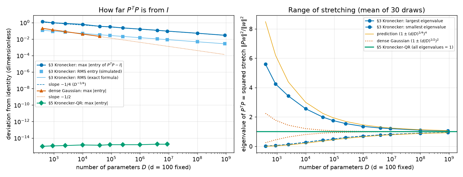
Figure: left, how far \(P^\top P\) is from \(I\) as \(D\) grows (\(d=100\); output [2]); right, the range of squared stretches \(\lVert Pw\rVert^2/\lVert w\rVert^2\), which are the eigenvalues of \(P^\top P\). The orange curves are a random-matrix prediction explained in the deeper block.
Three further pairs, with \(d\) growing along with \(D\), tell the same story: the mean largest deviation is 0.4813 at \((100^2,10^2)\), 0.3528 at \((300^2,20^2)\) and 0.2134 at \((1000^2,30^2)\) (output [2]).
Step 3: at the size of GPT-2 small. Take \(D=123{,}689{,}472\) (the nanoGPT parameter count used in Chapters 5 and 7; the paper never states the \(D\) of its subspace runs) and the paper's \(d=50{,}000\). The square parts are \(11{,}121^2=123{,}676{,}641\) and \(223^2=49{,}729\). Factors of shape \(11{,}121\times223\) are small enough to draw exactly, and Step 1 showed that \(P^\top P\) follows from them (output [3]):
- §3 projector: largest entry deviation 0.0772 (diagonal) and 0.0439 (off-diagonal); RMS \(9.07\times10^{-4}\) (exact formula \(9.05\times10^{-4}\)).
- But the stretch range is wide: eigenvalues of \(P^\top P\) in \([0.5512,\,1.6846]\), so \(\lVert Pw\rVert/\lVert w\rVert\) lies between 0.7424 and 1.2979, and the condition number is 3.06. A dense Gaussian matrix of the same size would give about \([0.9603,\,1.0405]\).
- §5 projector: \(\max\lvert P^\top P-I\rvert=5.0\times10^{-15}\).
- Storage: a dense \(P\) would hold \(6.184\times10^{12}\) numbers, 24.7 TB as 32-bit floats. The factors hold \(2\times11{,}121\times223=4{,}959{,}966\) numbers, 19.8 MB. One product \(Pw\) costs \(2.81\times10^{10}\) multiplications with the vec trick instead of \(6.18\times10^{12}\).
So "\(P^\top P\approx I\)" for the §3 recipe is true entry by entry, but at the paper's sizes some directions of \(w\) are still stretched 1.748 times as much as others (\(1.2979/0.7424\)). The §5 recipe removes this.
Step 4: why the stretch range matters for training. Take the quadratic loss \(L(w)=\tfrac12\lVert\theta_0+Pw-\theta^*\rVert^2\) with a random target \(\theta^*\), \(\theta_0=0\), and the three projectors of Step 1. Run gradient descent from \(w=0\) with the best constant learning rate for each matrix, and count the steps until \(w\) is within a millionth (relative) of the best point on the subspace (output [5]):
| Projector | eigenvalue range | condition number | steps |
|---|---|---|---|
| §3 Kronecker | [0.1008, 3.6878] | 36.59 | 196 |
| dense Gaussian | [0.6456, 1.4316] | 2.22 | 13 |
| §5 Kronecker-QR | [1.0000, 1.0000] | 1.00 | 1 |
With an orthonormal \(P\) the loss in \(w\) is as round as the loss in \(\theta\), and one step with learning rate 1 lands exactly on the optimum. With a badly conditioned \(P\), a learning rate small enough for the most-stretched direction is far too small for the most-squashed one. SOURCE: Lotfi et al. 2022, §4 This is what that paper means by choosing \(P\) approximately orthonormal "to facilitate favorable conditioning during optimization". MY EXPLANATION The paper trains with AdamW (Chapter 7), which rescales each coordinate of \(w\) separately. That partly compensates for unequal column lengths, but not for columns that are far from perpendicular, so this gradient-descent count is a model of the effect, not a prediction for AdamW.
Step 5: intrinsic dimension of a small network. A network with 10 inputs, two hidden layers of 32 units and 4 outputs has \(D=1{,}540\) parameters. It is trained on 600 examples labelled by a fixed random "teacher" network and tested on 4,000 fresh examples (output [6]).
- Before training at scale, the script checks the two mechanics: the vec trick reproduces the explicit \(Q_1\otimes Q_2\) to \(2.2\times10^{-16}\), and autograd's \(\nabla_w L\) equals \(P^\top\nabla_\theta L\) to \(6.2\times10^{-17}\).
- Training all 1,540 parameters reaches test accuracy 0.758 (training accuracy 1.000).
- Training only \(w\) in random subspaces (three dense-QR projectors per \(d\), plus one Kronecker-QR projector laid out as in the authors' code):
| \(d\) | test accuracy, dense-QR (mean; min–max) | train accuracy (mean) | test accuracy, Kronecker-QR | bits to store \(w\) (32-bit) |
|---|---|---|---|---|
| 2 | 0.238 (0.231–0.248) | 0.228 | 0.203 | 64 |
| 10 | 0.341 (0.283–0.375) | 0.363 | 0.362 | 320 |
| 20 | 0.521 (0.515–0.528) | 0.563 | 0.509 | 640 |
| 50 | 0.660 (0.646–0.670) | 0.762 | 0.679 | 1,600 |
| 100 | 0.705 (0.700–0.710) | 0.866 | 0.701 | 3,200 |
| 500 | 0.738 (0.735–0.740) | 1.000 | 0.736 | 16,000 |
Ninety percent of 0.758 is 0.682. The smallest \(d\) in the grid whose mean test accuracy reaches it is 100, so \(d_{\text{int90}}=100\) here: \(d/D=6.5\,\%\) of the parameters' worth of freedom, and 3,200 bits instead of 49,280. The largest class makes up 0.285 of the test set, so the \(d=2\) model is barely better than always guessing that class.
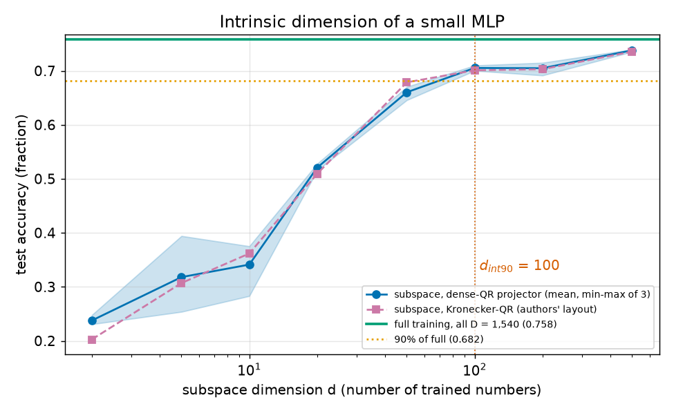
Figure: the intrinsic-dimension curve of the small network (output [6]). The Kronecker-QR projector performs like a dense one. SOURCE: Lotfi et al. 2022, Figure 2 They report the same for ResNets: Kronecker, sparse and dense projectors train almost identically, while the Kronecker one is far cheaper.
MY EXPLANATION The same trade-off appears in the paper. Reading the plotted points of Figure 1 (left) exactly
(fig_extract.py), the best "Subspace Only" BPD bound is 13.8138 bits/token of training loss plus 0.7758 of
complexity, total 14.5896. Its complexity is the smallest of the three methods, but its training loss is high. PAPER
Tables 1–2, pp. 6–7 The subspace-only GPT-2 small model has bound 14.59 and validation BPD 13.85, against 12.12
and 10.53 for SubLoRA and a random-guess level of \(\log_2 50{,}257=15.617\) bits/token (\(V=50{,}257\):
SOURCE: GPT-2 tokenizer; output [6]). MY EXPLANATION A linear subspace of affordable size is too few
avenues for a 124-million-parameter transformer; Chapter 20 shows how SubLoRA spends the same \(d\) numbers more
effectively.
Step 6: non-square sizes. Output [4], with \(P\) formed explicitly:
- Authors' layout, \(D=10{,}050=100^2+50\), \(d=410=20^2+10\): the remainder block is a \(50\times10\) Gaussian. \(\max\lvert P^\top P-I\rvert=0.368\) and eigenvalues in \([0.3958,\,1.9407]\): the 10 remainder directions are poorly conditioned, while the 400 Kronecker directions are exact.
- Authors' layout, \(D=10{,}005\), \(d=410\): the remainder block is \(5\times10\), with fewer rows than columns. \(P^\top P\) has 5 zero eigenvalues: five directions of \(w\) change nothing at all.
- Authors' layout, \(D=10{,}000\) (a perfect square), \(d=410\): the remainder block has 0 rows, so 10 columns of \(P\) are entirely zero. Ten coordinates of \(w\) are ignored.
- Authors' layout, \(D=10{,}050\), \(d=400\) (a perfect square): exact, \(1.3\times10^{-15}\).
- Pad-and-truncate, \(D=10{,}050\), \(d=410\) (build \(10{,}201\times441\)): dropping columns only is exact (\(1.4\times10^{-15}\)); dropping rows too gives \(\max\lvert P^\top P-I\rvert=0.0386\) and smallest eigenvalue 0.7857.
- A fix: QR-orthogonalize the remainder block as well (possible when it has at least as many rows as columns). Then \(P^\top P=I\) to \(1.1\times10^{-15}\).
At GPT-2 scale, pad-and-truncate would drop 9,412 of 123,698,884 rows. The script bounds the damage without forming \(P\): every entry of \(P^\top P-I\) is at most \(5.9\times10^{-4}\), and the smallest eigenvalue is at least \(1-0.0171\). Small, but not exact.
Going deeper¶
The derivations sit in the blocks below. Chapter 8 already proved the mixed-product property, the vec trick and the variances of Gaussian dot products; we use them without repeating the proofs.
Going deeper: the gradient through θ = θ0 + Pw, entry by entry
MY EXPLANATION Write \(\theta_i=(\theta_0)_i+\sum_{k=1}^dP_{ik}w_k\) for \(i=1,\dots,D\). Then \(\partial\theta_i/\partial w_k=P_{ik}\), because \(\theta_0\) and \(P\) are fixed numbers and only the term with \(w_k\) depends on \(w_k\). The loss depends on \(w\) only through \(\theta\), so the chain rule of calculus (Chapter 7) gives
The last step is the definition of the matrix–vector product with \(P^\top\), whose row \(k\) is column \(k\) of \(P\). Stacking over \(k\): \(\nabla_wL=P^\top\nabla_\theta L\). Output [6] checks this against autograd (\(6.2\times10^{-17}\)).
Step lengths. A gradient step changes \(w\) by \(\Delta w=-\eta\nabla_wL\) (\(\eta\) is the learning rate) and therefore \(\theta\) by \(\Delta\theta=P\Delta w\). If \(P^\top P=I\), \(\lVert\Delta\theta\rVert=\lVert\Delta w\rVert\): a learning rate means the same distance in both spaces. Otherwise \(\lVert\Delta\theta\rVert/\lVert\Delta w\rVert\) lies between \(\sqrt{\lambda_{\min}}\) and \(\sqrt{\lambda_{\max}}\) (next block).
Going deeper: stretch, eigenvalues, and the eigenvalues of a Kronecker product
MY EXPLANATION Let \(S=P^\top P\), a symmetric \(d\times d\) matrix (\(S^\top=S\)). A number \(\lambda\) is an eigenvalue of \(S\) with eigenvector \(u\ne0\) if \(Su=\lambda u\): \(S\) only rescales \(u\).
Spectral theorem (stated, proof skipped). Every real symmetric \(d\times d\) matrix can be written \(S=U\Lambda U^\top\) with \(U\) a \(d\times d\) matrix with orthonormal columns and \(\Lambda\) diagonal. The diagonal entries \(\lambda_1,\dots,\lambda_d\) are the eigenvalues, and column \(j\) of \(U\) is an eigenvector for \(\lambda_j\). The proof (by induction on \(d\), using that a symmetric matrix has a real eigenvalue) is standard and is not needed for anything else in this explainer.
Squared stretch = eigenvalue range. For \(w\ne0\) put \(c=U^\top w\). Since \(U\) is square with orthonormal columns, \(\lVert c\rVert=\lVert w\rVert\) (Chapter 8). Then
This is a weighted average of the \(\lambda_j\) with weights \(c_j^2\ge0\), so it lies between \(\lambda_{\min}\) and \(\lambda_{\max}\), and it reaches each extreme when \(w\) is the corresponding eigenvector. All \(\lambda_j\ge0\) because a squared length cannot be negative.
Eigenvalues of a Kronecker product are products of eigenvalues. Let \(F_1=U_1\Lambda_1U_1^\top\) and \(F_2=U_2\Lambda_2U_2^\top\). By the mixed-product property applied twice and the transpose rule,
\(U_1\otimes U_2\) has orthonormal columns (Chapter 8's corollary) and \(\Lambda_1\otimes\Lambda_2\) is diagonal with entries \(\lambda_i\mu_j\) (every eigenvalue of \(F_1\) times every eigenvalue of \(F_2\)). So these products are the eigenvalues of \(P^\top P=F_1\otimes F_2\). Since all are \(\ge0\), the extremes are \(\lambda_{\max}(F_1)\lambda_{\max}(F_2)\) and \(\lambda_{\min}(F_1)\lambda_{\min}(F_2)\). This is how the script gets the stretch range at GPT-2 scale from two \(223\times223\) matrices.
The orange curves in the figure. SOURCE: Marchenko and Pastur (1967), a classical random-matrix result; proof well beyond this explainer For a Gaussian matrix with \(a\) rows, \(b\) columns and \(\mathcal N(0,1/a)\) entries, with \(a\) and \(b\) large, the eigenvalues of its \(G^\top G\) fill the interval \([(1-\sqrt{b/a})^2,(1+\sqrt{b/a})^2]\). MY EXPLANATION Each \(F_i\) is such a matrix with \(a=\sqrt D\), \(b=\sqrt d\), so by the product rule above the stretch range of the §3 projector should be about \([(1-r)^4,(1+r)^4]\) with \(r=(d/D)^{1/4}\). At GPT-2 scale \(r=0.1416\), predicting \([0.5429,\,1.6985]\); the script measures \([0.5512,\,1.6846]\) (output [3]). A dense Gaussian \(D\times d\) matrix has \(r'=(d/D)^{1/2}=0.0201\) instead, a much narrower range. The point is that the stretch range depends on \((d/D)^{1/4}\), which for the paper's sizes is not small.
Going deeper: the exact RMS deviation of the §3 projector, and why it is D to the minus 1/4
MY EXPLANATION Throughout, \(D\) and \(d\) are fixed perfect squares; \(G_1,G_2\) are random with independent \(\mathcal N(0,1)\) entries; every expectation is over their draw.
Write \(s=\sqrt D\) and \(t=\sqrt d\) only inside this block. \(F_i=G_i^\top G_i/s\) is \(t\times t\). From Chapter 8's last deeper block, applied to a Gaussian matrix with \(s\) rows and entries of variance \(1/s\) (that is, \(G_i/\sqrt s\)):
- a diagonal entry \(F_{jj}\) has mean 1 and variance \(2/s\), so \(\mathbb E[F_{jj}^2]=1+2/s\);
- an off-diagonal entry \(F_{jk}\) (\(j\ne k\)) has mean 0 and variance \(1/s\), so \(\mathbb E[F_{jk}^2]=1/s\).
\(F_1\) and \(F_2\) are independent (built from independent matrices). Entry \(((j_1,j_2),(k_1,k_2))\) of \(P^\top P=F_1\otimes F_2\) is \((F_1)_{j_1k_1}(F_2)_{j_2k_2}\). There are three kinds of entries:
- Diagonal (\(j_1=k_1\), \(j_2=k_2\)), \(d\) of them. Expected squared deviation from 1: \(\mathbb E[(F_1)_{jj}^2]\,\mathbb E[(F_2)_{jj}^2]-2\,\mathbb E[(F_1)_{jj}]\,\mathbb E[(F_2)_{jj}]+1=(1+2/s)^2-1\).
- Mixed (exactly one factor on its diagonal), \(2\cdot t\cdot t(t-1)=2d(t-1)\) of them. Expected square: \((1+2/s)\cdot(1/s)\).
- Doubly off-diagonal, the remaining \(d(t-1)^2\) entries. Expected square: \((1/s)(1/s)=1/s^2\).
(Check: \(d+2d(t-1)+d(t-1)^2=d\,t^2=d^2\), all entries.) The mean of the squared entries of \(P^\top P-I\) is therefore
and the "exact formula" column of Step 2 is its square root. (Strictly, the square root of the expected mean square, not the expected RMS; the two agree closely here.) For large \(s\) the middle term dominates: \(\mathbb E[\text{MS}]\approx\frac{2(t+1)}{d}\cdot\frac1s\), so
For \(d=100\) the constant is \(\sqrt{0.22}=0.469\), and at \(D=10^6\) this gives \(0.0148\) (output [2]), against 0.01487 from the full formula and 0.01438 simulated. The mixed entries are products of one near-1 number and one \(D^{-1/4}\)-sized number, which is why the Kronecker structure converges only like \(D^{-1/4}\): each factor has only \(\sqrt D\) rows to average over.
The largest entry. The diagonal entries have standard deviation about \(2/\sqrt s=2D^{-1/4}\), and the largest of \(d\) such entries is a few standard deviations (it grows slowly with \(d\)). With \(d\) fixed, the largest entry therefore also scales like \(D^{-1/4}\), which the fitted slope \(-0.259\) confirms. We do not derive the constant.
Going deeper: why a better-conditioned P makes gradient descent faster
MY EXPLANATION Take \(L(w)=\tfrac12\lVert Pw-b\rVert^2\) for a fixed vector \(b\) (here \(b=\theta^*-\theta_0\)). Its gradient is \(\nabla_wL=P^\top(Pw-b)=Sw-P^\top b\) with \(S=P^\top P\). Assume \(S\) has \(\lambda_{\min}>0\). The best point \(w^*\) solves \(Sw^*=P^\top b\). Subtracting, the gradient step \(w_{t+1}=w_t-\eta\nabla_wL(w_t)\) gives
With \(S=U\Lambda U^\top\), the component of the error along eigenvector \(j\) is multiplied by \((1-\eta\lambda_j)\) at every step. The slowest component shrinks by \(\rho(\eta)=\max_j\lvert1-\eta\lambda_j\rvert\). This maximum is attained at \(\lambda_{\min}\) or \(\lambda_{\max}\), and it is smallest when the two are balanced, \(1-\eta\lambda_{\min}=\eta\lambda_{\max}-1\), that is, \(\eta=2/(\lambda_{\max}+\lambda_{\min})\). Then
The error after \(k\) steps is at most \(\rho^k\) times the starting error, so reaching a factor \(10^{-6}\) needs at most \(\lceil\ln(10^{-6})/\ln\rho\rceil\) steps. For \(\kappa=36.59\), \(\rho=0.9468\) and the bound is 253 steps; the run took 196 (output [5], "bound ~253"). For \(\kappa=1\), \(\rho=0\): one step, as observed. The \(\ln\) here is the natural log, but any base gives the same ratio.
Going deeper: what the authors' non-square layout does to PᵀP
[MY EXPLANATION, about SOURCE: authors' code RoundedDoubleKronQR] Write the layout as
\(P=\Pi\begin{pmatrix}K&0\\0&R\end{pmatrix}\), with \(K=Q_1\otimes Q_2\) of shape \(D_0\times d_0\), the remainder \(R\)
of shape \((D-D_0)\times(d-d_0)\), and \(\Pi\) a \(D\times D\) permutation matrix (it reorders rows; \(\Pi^\top\Pi=I\)
because each row and column has one 1). By block multiplication (Chapter 8),
So everything depends on the remainder. Three cases:
- \(R\) is Gaussian with \(\mathcal N(0,1/(D-D_0))\) entries and more rows than columns: \(R^\top R\approx I\) with the quality of a small dense Gaussian matrix, which can be poor (eigenvalues \([0.3958,1.9407]\) for \(50\times10\)).
- \(R\) has fewer rows than columns: \(\operatorname{rank}R\le D-D_0<d-d_0\) (Chapter 8, fact 1), so \(R^\top R\) is singular: at least \((d-d_0)-(D-D_0)\) directions of \(w\) satisfy \(Pw=0\). Output [4]: 5 zero eigenvalues for a \(5\times10\) remainder.
- \(D\) is a perfect square but \(d\) is not: \(R\) has no rows, so its \(d-d_0\) columns of \(P\) are zero.
\(D-D_0\) is at most \(2\lfloor\sqrt D\rfloor\) and \(d-d_0\) at most \(2\lfloor\sqrt d\rfloor\) (because \((x+1)^2=x^2+2x+1\)), so the remainder is small compared with \(P\). Whether the paper's runs hit a bad case depends on the SubLoRA parameter count \(D\), which the paper does not report.
Pad-and-truncate. If \(\tilde P\) has orthonormal columns and we keep rows \(\mathcal K\) and drop rows \(\mathcal R\), then \(I=\tilde P^\top\tilde P=\tilde P_{\mathcal K}^\top\tilde P_{\mathcal K}+\tilde P_{\mathcal R}^\top\tilde P_{\mathcal R}\) (block multiplication by rows), so the kept matrix has \(P^\top P=I-\tilde P_{\mathcal R}^\top\tilde P_{\mathcal R}\). The error is the Gram matrix of the dropped rows. At GPT-2 scale the dropped rows are the last 9,412 rows of one block, which in Kronecker form are \(q^\top\otimes(\text{last 9,412 rows of }Q_2)\) with \(q\) the last row of \(Q_1\), so the error equals \((qq^\top)\otimes M\) restricted to the kept columns, with \(M\) the Gram matrix of those rows of \(Q_2\). Its largest entry and largest eigenvalue are at most those of \((qq^\top)\otimes M\), namely \(\max\lvert q_jq_k\rvert\max\lvert M\rvert=5.9\times10^{-4}\) and \(\lVert q\rVert^2\lambda_{\max}(M)=0.0171\) (output [4]). Restricting to kept columns can only lower both, because it takes a principal submatrix.
Code note (listed under the notes on the authors' code in the errata page): the authors' remainder block can switch off directions of w
[SOURCE: authors' code, sublora_nn_projectors.py, RoundedDoubleKronQR] This is about the released code,
not an error in the paper. MY EXPLANATION As shown above, when \(D-D_0<d-d_0\) the remainder block makes
\(P^\top P\) singular, and when \(D\) is a perfect square and \(d\) is not, \(d-d_0\) columns of \(P\) are zero. The
corresponding coordinates of \(w\) are still quantized and coded (they cost bits) but cannot change the model.
Separately, the remainder block is plain Gaussian, so even in the good case \(P^\top P\ne I\) on it. QR-orthogonalizing
the remainder (when it has at least as many rows as columns) makes \(P^\top P=I\) exactly (output [4]). The effect
on the paper's numbers is unknown, because the paper does not state \(D\); it can only make the reported models
slightly worse, never make a bound invalid, since the bound holds for whatever \(P\) was fixed in advance.
Common misconceptions¶
- Misconception: "Training in a \(d\)-dimensional subspace gives a smaller model with \(d\) parameters." — Actually: the network keeps all \(D\) parameters and every forward pass uses them. Only \(d\) numbers are free; the other \(D-d\) degrees of freedom are fixed by \(\theta_0\) and \(P\). That is why the description is short but the computation is not cheaper.
- Misconception: "The subspace passes through the origin, so the model starts at all-zero weights." — Actually: it is an affine subspace through the random initialization \(\theta_0\); \(w=0\) means \(\theta=\theta_0\), an ordinary randomly initialized network.
- Misconception: "The §3 recipe gives \(P^\top P\approx I\), so it is as good as orthonormal." — Actually: the deviation shrinks only like \(D^{-1/4}\) (fitted slope \(-0.259\)). At \(D=10{,}000\), \(d=400\) its stretch range is \([0.1008,3.6878]\) (condition number 36.59, 196 gradient steps vs 1 for QR); even at GPT-2 scale with \(d=50{,}000\) the condition number is 3.06. The §5 QR recipe is exact.
- Misconception: "Small entries of \(P^\top P-I\) mean all directions are treated equally." — Actually: at GPT-2 scale every entry is below 0.08, yet \(\lVert Pw\rVert/\lVert w\rVert\) ranges from 0.7424 to 1.2979. Many small errors add up along special directions; the eigenvalue range is the right measure.
- Misconception: "Rounding non-square sizes is a harmless implementation detail." — Actually: dropping rows breaks exact orthonormality (smallest eigenvalue 0.7857 in Step 6), and the authors' block layout can create directions of \(w\) that do nothing (5 zero eigenvalues at \(D=10{,}005\), \(d=410\)).
- Misconception: "A useful subspace must have \(d\) close to \(D\)." — Actually: in Step 5, \(d=100\) of
\(D=1{,}540\) reaches 90 % of full-training accuracy; the paper's best GPT-2 small bound appears to use \(d=50{,}000\)
for about 124 million parameters (read from the plotted points of Figure 2, left; Chapter 20, output [4] of
ch20_sublora.py). How small \(d\) can be depends on the task (intrinsic dimension).
Self-test¶
Q1. A projector has eigenvalues of \(P^\top P\) between 0.1008 and 3.6878. Using gradient descent with the best constant learning rate on \(L(w)=\tfrac12\lVert Pw-b\rVert^2\), at most how many steps reduce the error by a factor \(10^{6}\)? How many does an exactly orthonormal \(P\) need?
Answer
\(\kappa=3.6878/0.1008=36.59\) and \(\rho=(\kappa-1)/(\kappa+1)=0.9468\). Each step multiplies the worst error component by at most \(\rho\), so the number of steps is at most \(\lceil\ln(10^{-6})/\ln\rho\rceil=253\) (output [5]; the actual run took 196). With \(P^\top P=I\), the learning rate \(\eta=1\) gives \(w_1-w^*=(I-I)(w_0-w^*)=0\): one step.
Q2. Pad-and-truncate builds an orthonormal matrix that is slightly too big and then cuts it. Why does cutting columns keep \(P^\top P=I\) while cutting rows breaks it?
Answer
\(P^\top P\) collects dot products between columns. Cutting columns removes some of these dot products but leaves the others unchanged: the remaining columns are still unit vectors and still perpendicular. Cutting rows changes every column: each one loses some entries, so its length drops below 1 and two columns' dot product loses the terms from the dropped rows. Precisely, \(P^\top P=I-\tilde P_{\mathcal R}^\top\tilde P_{\mathcal R}\), where \(\tilde P_{\mathcal R}\) are the dropped rows. In Step 6 this gives a smallest eigenvalue of 0.7857.
Q3. In the authors' layout, \(D=10{,}005=100^2+5\) and \(d=410=20^2+10\). How many coordinates of \(w\) can change the model, and why? What changes if \(D=10{,}000\)?
Answer
The Kronecker block handles 400 coordinates exactly. The remaining 10 coordinates go through a \(5\times10\) remainder block, whose rank is at most 5. So at least \(10-5=5\) directions of \(w\) give \(Pw=0\), and at most 405 independent directions of \(w\) affect \(\theta\) (output [4] finds exactly 5 zero eigenvalues). If \(D=10{,}000\) is a perfect square, the remainder has 0 rows, so 10 columns of \(P\) are zero and those 10 coordinates are ignored entirely (output [4]: 10 all-zero columns). In both cases the ignored coordinates still have to be stored.
Code for this chapter¶
Run it from the project root (it runs in under a minute on an idle laptop CPU; the wall times it prints depend on the machine):
.venv/Scripts/python explainer/code/ch18_subspace.py
Source: ch18_subspace.py
"""Chapter 18 demo -- random subspace training, theta = theta0 + P w.

Claims reproduced / checked (every number quoted in Chapter 18 is printed here):
  [1] D = 100^2, d = 20^2, P formed explicitly: the paper's §3 projector P = (G1 (x) G2)/sqrt(D)
      (G_i standard Gaussian, sqrt(D) x sqrt(d)) is only approximately orthonormal; the §5 projector
      P = Q1 (x) Q2 (Q_i = QR factors) is orthonormal to rounding error. P^T P computed explicitly
      equals the factor formula (G1^T G1 (x) G2^T G2)/D (mixed-product property). Storage counts.
  [2] Lotfi et al. (2022, §4.1) claim P^T P = I + O(D^(-1/4)) for the §3 projector: deviation vs D
      (fixed d = 100, 30 draws), fitted log-log slope, exact expected RMS formula, dense Gaussian
      comparison (~D^(-1/2)), QR version (~1e-15), and three further (D, d) pairs.
  [3] GPT-2 scale, exact without forming P: D = nanoGPT GPT-2-small count, d = 50,000 rounded to
      squares; deviation, eigenvalue range of P^T P, storage and multiplication counts.
  [4] Non-square D, d: the authors' code (block-diagonal Kronecker-QR part + dense Gaussian
      remainder, rows permuted), its degenerate cases, pad-and-truncate, and a QR-remainder fix.
  [5] Why orthonormality matters: the condition number of P^T P and the number of gradient-descent
      steps on a quadratic loss for the three projectors (D = 10,000, d = 400).
  [6] Gradients flow as grad_w L = P^T grad_theta L (autograd check with a vec-trick projector);
      intrinsic-dimension curve of a small MLP on a synthetic task, dense-QR vs Kronecker-QR.
Figures: explainer/docs/assets/fig/ch18_ptp_error.png, ch18_intrinsic_dim.png
Deterministic (numpy default_rng / torch.manual_seed); CPU only; runs in well under 60 s.
"""
from __future__ import annotations

import math
import sys
import time
from pathlib import Path

import numpy as np
import torch
import matplotlib

matplotlib.use("Agg")
import matplotlib.pyplot as plt  # noqa: E402

HERE = Path(__file__).resolve().parent
sys.path.insert(0, str(HERE))
import pacbound  # noqa: E402

OUT_TXT = HERE / "outputs" / "ch18_subspace.txt"
FIG_DIR = HERE.parent / "docs" / "assets" / "fig"
FIG_PTP = FIG_DIR / "ch18_ptp_error.png"
FIG_ID = FIG_DIR / "ch18_intrinsic_dim.png"

_lines: list[str] = []
T0 = time.time()


def out(s: str = "") -> None:
    print(s)
    _lines.append(s)


# ---------------------------------------------------------------------------
# helpers
# ---------------------------------------------------------------------------
def qr_q(G: np.ndarray) -> np.ndarray:
    """Q factor (orthonormal columns) of a tall matrix G."""
    Q, _ = np.linalg.qr(G, mode="reduced")
    return Q


def kron_stats(F1: np.ndarray, F2: np.ndarray) -> dict:
    """Deviation of S = F1 (x) F2 from the identity, computed from the small factors only.
    Entry ((j1,j2),(k1,k2)) of S is F1[j1,k1] * F2[j2,k2]."""
    d1, d2 = np.diag(F1), np.diag(F2)
    diag_dev = np.max(np.abs(np.outer(d1, d2) - 1.0))
    off1 = F1 - np.diag(d1)
    off2 = F2 - np.diag(d2)
    max_off = max(np.max(np.abs(off1)) * np.max(np.abs(F2)),
                  np.max(np.abs(d1)) * np.max(np.abs(off2)))
    d = F1.shape[0] * F2.shape[0]
    frob2 = (np.sum(F1 ** 2) * np.sum(F2 ** 2) - 2.0 * np.trace(F1) * np.trace(F2) + d)
    rms = math.sqrt(max(frob2, 0.0) / d ** 2)
    l1, l2 = np.linalg.eigvalsh(F1), np.linalg.eigvalsh(F2)
    lmax, lmin = l1.max() * l2.max(), l1.min() * l2.min()
    return dict(diag=diag_dev, off=max_off, max=max(diag_dev, max_off), rms=rms,
                lmax=lmax, lmin=lmin, cond=lmax / lmin)


def explicit_stats(S: np.ndarray) -> dict:
    d = S.shape[0]
    E = S - np.eye(d)
    diag_dev = np.max(np.abs(np.diag(E)))
    max_off = np.max(np.abs(E - np.diag(np.diag(E))))
    lam = np.linalg.eigvalsh(S)
    return dict(diag=diag_dev, off=max_off, max=max(diag_dev, max_off),
                rms=float(np.sqrt(np.mean(E ** 2))), lmax=lam.max(), lmin=lam.min(),
                cond=lam.max() / lam.min() if lam.min() > 1e-12 else float("inf"), eig=lam)


def rms_theory(sD: int, sd: int) -> float:
    """Exact expected mean of (P^T P - I)^2 over all d^2 entries, §3 projector, then sqrt.
    Diagonal: E[F1jj^2 F2jj^2] - 1 = (1 + 2/sD)^2 - 1; mixed: (1 + 2/sD)/sD; doubly-off: 1/sD^2."""
    d = sd * sd
    ms = (d * ((1 + 2 / sD) ** 2 - 1) + 2 * d * (sd - 1) * (1 + 2 / sD) / sD
          + d * (sd - 1) ** 2 / sD ** 2) / d ** 2
    return math.sqrt(ms)


# ===========================================================================
out("== Chapter 18: random subspace training, theta = theta0 + P w ==")
# [1] explicit small case
# ===========================================================================
rng = np.random.default_rng(0)
sD, sd = 100, 20
D, d = sD * sD, sd * sd
G1, G2 = rng.standard_normal((sD, sd)), rng.standard_normal((sD, sd))
P3 = np.kron(G1, G2) / math.sqrt(D)                 # §3 recipe, formed explicitly (10,000 x 400)
S3 = P3.T @ P3
S3_fac = np.kron(G1.T @ G1, G2.T @ G2) / D           # mixed-product property
Q1, Q2 = qr_q(G1), qr_q(G2)
P5 = np.kron(Q1, Q2)                                 # §5 recipe
S5 = P5.T @ P5
Gd = rng.standard_normal((D, d)) / math.sqrt(D)      # dense Gaussian N(0, 1/D), for contrast
Sd = Gd.T @ Gd
e3, e5, ed = explicit_stats(S3), explicit_stats(S5), explicit_stats(Sd)
f3 = kron_stats(G1.T @ G1 / sD, G2.T @ G2 / sD)
out(f"[1] D = {sD}^2 = {D:,}, d = {sd}^2 = {d}; P formed explicitly ({D:,} x {d})")
out(f"    explicit P^T P vs factor formula (G1^T G1 (x) G2^T G2)/D: max difference {np.max(np.abs(S3 - S3_fac)):.1e}")
out("    projector                         max|diag-1|  max|offdiag|  RMS(P^T P - I)  eig range of P^T P")
for name, e in [("§3 (G1 (x) G2)/sqrt(D)", e3), ("§5 Q1 (x) Q2 (QR factors)", e5),
                ("dense Gaussian N(0,1/D)", ed)]:
    out(f"    {name:33s} {e['diag']:.2e}     {e['off']:.2e}      {e['rms']:.2e}        "
        f"[{e['lmin']:.4f}, {e['lmax']:.4f}]")
out(f"    factor-only formulas reproduce the explicit §3 numbers: max {f3['max']:.4e} vs {e3['max']:.4e}; "
    f"eig [{f3['lmin']:.4f}, {f3['lmax']:.4f}]")
w = rng.standard_normal(d)
out(f"    ||w|| = {np.linalg.norm(w):.4f}; ||P w||: §3 {np.linalg.norm(P3 @ w):.4f}, §5 {np.linalg.norm(P5 @ w):.4f}, "
    f"dense {np.linalg.norm(Gd @ w):.4f}")
Qs = qr_q(G1 / sD ** 0.5)       # scale 1/D^(1/4) = std of N(0, 1/sqrt(D)) read as a variance
out(f"    QR ignores scale: Q of G1 vs Q of G1/D^(1/4): max difference {np.max(np.abs(Qs - Q1)):.1e}")
out(f"    §3 stretch ||Pw||/||w|| ranges over [sqrt(lmin), sqrt(lmax)] = [{math.sqrt(e3['lmin']):.2f}, "
    f"{math.sqrt(e3['lmax']):.2f}]")
out(f"    storage: dense P {D * d:,} numbers; Kronecker factors 2 x {sD} x {sd} = {2 * sD * sd:,} numbers")

# ===========================================================================
# [2] deviation vs D for the §3 projector (Lotfi et al. 2022: O(D^-1/4))
# ===========================================================================
out("[2] §3 projector, d = 10^2 fixed, 30 draws per D (means); dense Gaussian: 10 draws (4 for D >= 10^4); QR: 3 draws")
SD_LIST = [20, 30, 50, 100, 200, 300, 500, 1000, 2000, 3000, 10000, 30000]
SD_SMALL = 10
NDRAW = 30
rng = np.random.default_rng(1)
sweep = []
for s in SD_LIST:
    st = []
    for _ in range(NDRAW):
        A = rng.standard_normal((s, SD_SMALL))
        B = rng.standard_normal((s, SD_SMALL))
        st.append(kron_stats(A.T @ A / s, B.T @ B / s))
    row = {k: float(np.mean([x[k] for x in st])) for k in ("diag", "off", "max", "rms", "lmax", "lmin")}
    qr_max = 0.0
    if s <= 3000:
        for _ in range(3):
            QA = qr_q(rng.standard_normal((s, SD_SMALL)))
            QB = qr_q(rng.standard_normal((s, SD_SMALL)))
            qr_max = max(qr_max, kron_stats(QA.T @ QA, QB.T @ QB)["max"])
    row.update(sD=s, D=s * s, qr=qr_max if s <= 3000 else float("nan"), rms_th=rms_theory(s, SD_SMALL))
    sweep.append(row)
out("       D            mean max|P^TP-I|  (diag / off)        RMS     RMS theory   D^(-1/4)   QR max")
for r in [r for r in sweep if r["sD"] in (20, 50, 100, 300, 1000, 3000, 10000, 30000)]:
    qr_txt = f"{r['qr']:.1e}" if not math.isnan(r["qr"]) else "   -   "
    out(f"    {r['D']:>13,}   {r['max']:.4f}   ({r['diag']:.4f} / {r['off']:.4f})   {r['rms']:.5f}  {r['rms_th']:.5f}"
        f"      {r['D'] ** -0.25:.4f}    {qr_txt}")
big = [r for r in sweep if r["sD"] >= 100]
slope_max = np.polyfit(np.log([r["D"] for r in big]), np.log([r["max"] for r in big]), 1)[0]
slope_rms = np.polyfit(np.log([r["D"] for r in big]), np.log([r["rms"] for r in big]), 1)[0]
out(f"    fitted log-log slope for D >= 10^4: max deviation {slope_max:.3f}, RMS {slope_rms:.3f}  (D^(-1/4) -> -0.25)")
c_rms = math.sqrt(2 * (SD_SMALL + 1) / SD_SMALL ** 2)
out(f"    large-D RMS ~ sqrt(2(sqrt d + 1)/d) D^(-1/4) = {c_rms:.3f} D^(-1/4); at D = 10^6: {c_rms * 1e6 ** -0.25:.4f}")
assert abs(slope_max + 0.25) < 0.03 and abs(slope_rms + 0.25) < 0.03
dense_rows = []
for s in [20, 30, 50, 100, 200]:
    vals = []
    for _ in range(10 if s <= 50 else 4):
        Gx = rng.standard_normal((s * s, 100)) / s
        vals.append(np.max(np.abs(Gx.T @ Gx - np.eye(100))))
    dense_rows.append((s * s, float(np.mean(vals))))
out("    dense Gaussian D x 100, N(0,1/D), mean max|P^TP-I|: "
    + ", ".join(f"D={D_:,}: {v:.4f}" for D_, v in dense_rows))
sl_dense = np.polyfit(np.log([x[0] for x in dense_rows]), np.log([x[1] for x in dense_rows]), 1)[0]
out(f"    dense fitted slope {sl_dense:.3f} (D^(-1/2) -> -0.5)")
out("    three further (D, d) pairs with growing d (30 draws, mean):")
for s, t in [(100, 10), (300, 20), (1000, 30)]:
    st = []
    for _ in range(NDRAW):
        A = rng.standard_normal((s, t))
        B = rng.standard_normal((s, t))
        st.append(kron_stats(A.T @ A / s, B.T @ B / s))
    mx = np.mean([x["max"] for x in st]); rm = np.mean([x["rms"] for x in st])
    out(f"      D = {s}^2 = {s * s:>9,}, d = {t}^2 = {t * t:>4}: max {mx:.4f}, RMS {rm:.5f} "
        f"(theory {rms_theory(s, t):.5f}), D^(-1/4) = {(s * s) ** -0.25:.4f}")

# ===========================================================================
# [3] GPT-2 scale, exact through the factors
# ===========================================================================
D_G = pacbound.gpt2_params(12, 768)            # nanoGPT count (Chapters 5, 7); the paper does not state D
d_G = 50_000                                   # [PAPER Fig. 2 / App. E] the d of the best GPT-2-small bound
sDg, sdg = math.isqrt(D_G), math.isqrt(d_G)
rng = np.random.default_rng(2)
A = rng.standard_normal((sDg, sdg)); B = rng.standard_normal((sDg, sdg))
g3 = kron_stats(A.T @ A / sDg, B.T @ B / sDg)
QA, QB = qr_q(A), qr_q(B)
g5 = kron_stats(QA.T @ QA, QB.T @ QB)
ratio = math.sqrt(sdg / sDg)                    # Marchenko-Pastur edges (1 +/- sqrt(cols/rows))^2 per factor
out(f"[3] GPT-2 scale: D = {D_G:,} (nanoGPT count, Ch. 5/7) -> square part floor(sqrt D)^2 = {sDg}^2 = {sDg ** 2:,}"
    f" (remainder {D_G - sDg ** 2:,} rows)")
out(f"    d = {d_G:,} -> square part {sdg}^2 = {sdg ** 2:,} (remainder {d_G - sdg ** 2} columns); factors {sDg:,} x {sdg}")
out(f"    §3 projector: max|diag-1| = {g3['diag']:.4f}, max|offdiag| = {g3['off']:.4f}, RMS = {g3['rms']:.2e} "
    f"(theory {rms_theory(sDg, sdg):.2e}); D0^(-1/4) = {(sDg ** 2) ** -0.25:.4f}")
out(f"      eigenvalues of P^T P in [{g3['lmin']:.4f}, {g3['lmax']:.4f}], condition number {g3['cond']:.2f}; "
    f"||Pw||/||w|| in [{math.sqrt(g3['lmin']):.4f}, {math.sqrt(g3['lmax']):.4f}] "
    f"(ratio {math.sqrt(g3['lmax'] / g3['lmin']):.3f})")
out(f"      Marchenko-Pastur prediction [(1-r)^4, (1+r)^4], r = (d0/D0)^(1/4) = {ratio:.4f}: "
    f"[{(1 - ratio) ** 4:.4f}, {(1 + ratio) ** 4:.4f}]")
rd = math.sqrt(sdg ** 2 / sDg ** 2)
out(f"      a dense Gaussian of the same size would give [(1-r')^2, (1+r')^2], r' = (d0/D0)^(1/2) = {rd:.4f}: "
    f"[{(1 - rd) ** 2:.4f}, {(1 + rd) ** 2:.4f}]")
out(f"    §5 projector (QR factors): max|P^T P - I| = {g5['max']:.1e}")
out(f"    storage: dense P = {D_G * d_G:.3e} numbers = {4 * D_G * d_G / 1e12:.1f} TB (float32, 1 TB = 1e12 bytes); "
    f"factors 2 x {sDg:,} x {sdg} = {2 * sDg * sdg:,} numbers = {8 * sDg * sdg / 1e6:.1f} MB")
out(f"    multiplications for Pw: dense D d = {D_G * d_G:.2e}; vec trick d0 sqrt(D0) + D0 sqrt(d0) = "
    f"{sdg ** 2 * sDg + sDg ** 2 * sdg:.2e}")

# ===========================================================================
# [4] non-square D, d
# ===========================================================================
def authors_projector(D: int, d: int, rng: np.random.Generator) -> np.ndarray:
    """Explicit version of RoundedDoubleKronQR (authors' code, sublora_nn_projectors.py):
    [Kron-QR block (floor(sqrt D)^2 x floor(sqrt d)^2)] (+) [dense Gaussian remainder], block-diagonal,
    then a random row permutation."""
    s, t = math.isqrt(D), math.isqrt(d)
    K = np.kron(qr_q(rng.standard_normal((s, t))), qr_q(rng.standard_normal((s, t))))
    rr, rc = D - s * s, d - t * t
    if rr == 0 or rc == 0:
        R = rng.standard_normal((rr, rc)) / math.sqrt(D)          # code: randn / sqrt(D)
    else:
        R = rng.standard_normal((rr, rc)) / math.sqrt(rr)         # code: LazyRandom(rr, rc) -> randn / sqrt(rr)
    P = np.zeros((D, d))
    P[: s * s, : t * t] = K
    P[s * s:, t * t:] = R
    return P[rng.permutation(D)]


def describe(P: np.ndarray) -> str:
    e = explicit_stats(P.T @ P)
    nzero = int(np.sum(np.linalg.norm(P, axis=0) == 0))
    nnull = int(np.sum(e["eig"] < 1e-10))
    return (f"max|P^TP-I| = {e['max']:.3e}, eig range [{e['lmin']:.4f}, {e['lmax']:.4f}], "
            f"zero eigenvalues {nnull}, all-zero columns {nzero}")


rng = np.random.default_rng(3)
out("[4] non-square D, d (P formed explicitly)")
for D_, d_ in [(10_050, 410), (10_005, 410), (10_000, 410), (10_050, 400)]:
    s, t = math.isqrt(D_), math.isqrt(d_)
    out(f"    authors' layout, D = {D_:,} = {s}^2+{D_ - s * s}, d = {d_} = {t}^2+{d_ - t * t}: "
        f"{describe(authors_projector(D_, d_, rng))}")
D_, d_ = 10_050, 410
S_, T_ = math.isqrt(D_ - 1) + 1, math.isqrt(d_ - 1) + 1
K = np.kron(qr_q(rng.standard_normal((S_, T_))), qr_q(rng.standard_normal((S_, T_))))
out(f"    pad-and-truncate, D = {D_:,}, d = {d_}: build {S_}^2 x {T_}^2 = {S_ * S_:,} x {T_ * T_}, keep first {D_:,} rows "
    f"and {d_} columns")
out(f"      drop columns only: {describe(K[:, :d_])}")
out(f"      drop rows too    : {describe(K[:D_, :d_])}")
s, t = math.isqrt(D_), math.isqrt(d_)
Kf = np.kron(qr_q(rng.standard_normal((s, t))), qr_q(rng.standard_normal((s, t))))
Pf = np.zeros((D_, d_)); Pf[: s * s, : t * t] = Kf
Pf[s * s:, t * t:] = qr_q(rng.standard_normal((D_ - s * s, d_ - t * t)))
out(f"    fix (QR the remainder block too; needs remainder rows >= columns): {describe(Pf)}")
# truncation at GPT-2 scale: dropped rows are the last ones of the last block of Q1 (x) Q2
S_, T_ = math.isqrt(D_G - 1) + 1, math.isqrt(d_G - 1) + 1
ndrop = S_ * S_ - D_G
rng = np.random.default_rng(4)
q1 = qr_q(rng.standard_normal((S_, T_))); q2 = qr_q(rng.standard_normal((S_, T_)))
qlast = q1[-1]                                    # row index i1 = S-1 of Q1
M = q2[S_ - ndrop:].T @ q2[S_ - ndrop:]           # Gram matrix of the dropped rows of Q2
assert ndrop <= S_
dev_max = np.max(np.abs(np.outer(qlast, qlast))) * np.max(np.abs(M))
dev_spec = float(qlast @ qlast) * np.linalg.eigvalsh(M).max()
out(f"    GPT-2 scale pad-and-truncate: {S_:,}^2 = {S_ * S_:,} rows, drop {ndrop:,}; {T_}^2 = {T_ * T_:,} columns, "
    f"drop {T_ * T_ - d_G}")
out(f"      max|P^TP-I| <= {dev_max:.1e}; smallest eigenvalue >= 1 - {dev_spec:.4f}  (one direction shrinks)")
out("    [PAPER App. E] d grid, square part + remainder columns: "
    + "; ".join(f"{x:,} = {math.isqrt(x)}^2 + {x - math.isqrt(x) ** 2}" for x in pacbound.D_GRID))

# ===========================================================================
# [5] conditioning: GD steps on a quadratic, D = 10,000, d = 400
# ===========================================================================
rng = np.random.default_rng(5)
theta_star = rng.standard_normal(D)


def gd_steps(P: np.ndarray, lr: float, tol: float = 1e-6, cap: int = 100_000) -> int:
    """GD on L(w) = 0.5 ||P w - theta*||^2 from w = 0; steps until ||w - w*|| <= tol ||w*||."""
    H = P.T @ P
    b = P.T @ theta_star
    w_star = np.linalg.solve(H, b)
    w = np.zeros(P.shape[1])
    for k in range(1, cap + 1):
        w = w - lr * (H @ w - b)
        if np.linalg.norm(w - w_star) <= tol * np.linalg.norm(w_star):
            return k
    return cap


out("[5] conditioning (D = 10,000, d = 400), GD on L(w) = 0.5 ||theta0 + P w - theta*||^2, theta0 = 0,")
out("    best constant learning rate 2/(lmax + lmin); steps until ||w - w*|| <= 1e-6 ||w*||")
for name, P_ in [("§3 Kronecker (Gaussian)", P3), ("dense Gaussian", Gd), ("§5 Kronecker-QR", P5)]:
    lam = np.linalg.eigvalsh(P_.T @ P_)
    lr = 2.0 / (lam.max() + lam.min())
    kappa = lam.max() / lam.min()
    rate = (kappa - 1) / (kappa + 1)
    pred = math.ceil(math.log(1e-6) / math.log(rate)) if rate > 0 else 1
    out(f"    {name:24s} eig [{lam.min():.4f}, {lam.max():.4f}], condition number {kappa:7.2f}, "
        f"rho = (k-1)/(k+1) = {rate:.4f}, steps {gd_steps(P_, lr):5d} (bound ~{pred})")

# ===========================================================================
# [6] gradient check and intrinsic dimension of a small MLP
# ===========================================================================
torch.manual_seed(0)
torch.set_num_threads(4)
DT = torch.float64
N_IN, H1, H2, N_CLS = 10, 32, 32, 4
SHAPES = [(H1, N_IN), (H1,), (H2, H1), (H2,), (N_CLS, H2), (N_CLS,)]
D_MLP = sum(int(np.prod(s)) for s in SHAPES)


def unflatten(theta):
    parts, i = [], 0
    for s in SHAPES:
        n = int(np.prod(s))
        parts.append(theta[i:i + n].view(*s)); i += n
    return parts


def mlp(theta, x):
    W1, b1, W2, b2, W3, b3 = unflatten(theta)
    h = torch.relu(x @ W1.T + b1)
    h = torch.relu(h @ W2.T + b2)
    return h @ W3.T + b3


# synthetic task: labels from a random "teacher" network
g = torch.Generator().manual_seed(0)
TW1 = torch.randn(32, N_IN, generator=g, dtype=DT) / math.sqrt(N_IN)
TW2 = torch.randn(N_CLS, 32, generator=g, dtype=DT) / math.sqrt(32)


def make_data(n):
    x = torch.randn(n, N_IN, generator=g, dtype=DT)
    y = (torch.tanh(x @ TW1.T * 2.0) @ TW2.T).argmax(1)
    return x, y


N_TR, N_TE = 600, 4000
Xtr, Ytr = make_data(N_TR)
Xte, Yte = make_data(N_TE)


def init_theta(seed):
    gg = torch.Generator().manual_seed(seed)
    parts = []
    for s in SHAPES:
        if len(s) == 2:
            parts.append(torch.randn(*s, generator=gg, dtype=DT) * math.sqrt(2.0 / s[1]))
        else:
            parts.append(torch.zeros(*s, dtype=DT))
    return torch.cat([p.reshape(-1) for p in parts])


THETA0 = init_theta(137)
loss_fn = torch.nn.CrossEntropyLoss()


def accuracy(theta, x, y):
    with torch.no_grad():
        return float((mlp(theta, x).argmax(1) == y).double().mean())


STEPS, LR_FULL, LR_SUB = 400, 1e-2, 1e-1


def train_full():
    v = THETA0.clone().float().requires_grad_(True)
    x, y = Xtr.float(), Ytr
    opt = torch.optim.Adam([v], lr=LR_FULL)
    for _ in range(STEPS):
        opt.zero_grad()
        loss_fn(mlp(v, x), y).backward()
        opt.step()
    th = v.detach().double()
    return accuracy(th, Xtr, Ytr), accuracy(th, Xte, Yte)


def mlp_batched(thetas, x):
    """K networks at once: thetas is K x D, x is n x N_IN; returns K x n x N_CLS logits."""
    K, i, parts = thetas.shape[0], 0, []
    for s in SHAPES:
        n = int(np.prod(s))
        parts.append(thetas[:, i:i + n].reshape(K, *s)); i += n
    W1, b1, W2, b2, W3, b3 = parts
    h = torch.relu(torch.einsum("ni,khi->knh", x, W1) + b1[:, None, :])
    h = torch.relu(torch.einsum("kni,khi->knh", h, W2) + b2[:, None, :])
    return torch.einsum("kni,kci->knc", h, W3) + b3[:, None, :]


def train_subspaces(Ps):
    """Train K subspace models in one batched computation. Ps: list of D x d_k projectors;
    each is padded with zero columns to a common width (zero columns get zero gradient, so
    Adam never moves those coordinates of w)."""
    K, dmax = len(Ps), max(P.shape[1] for P in Ps)
    Pall = torch.zeros(K, D_MLP, dmax)
    for k, P in enumerate(Ps):
        Pall[k, :, : P.shape[1]] = torch.as_tensor(P, dtype=torch.float32)
    W = torch.zeros(K, dmax, requires_grad=True)
    th0, x = THETA0.float(), Xtr.float()
    yk = Ytr.repeat(K)
    opt = torch.optim.Adam([W], lr=LR_SUB)
    for _ in range(STEPS):
        opt.zero_grad()
        th = th0 + torch.einsum("kDd,kd->kD", Pall, W)
        logits = mlp_batched(th, x)
        # sum over runs of each run's mean loss: runs do not interact
        (loss_fn(logits.reshape(-1, N_CLS), yk) * K).backward()
        opt.step()
    th = (th0 + torch.einsum("kDd,kd->kD", Pall, W)).detach().double()
    return [(accuracy(th[k], Xtr, Ytr), accuracy(th[k], Xte, Yte)) for k in range(K)]


# gradient check with a vec-trick Kronecker-QR projector (D' = 39^2 rows used, d = 5^2)
s_, t_ = 39, 5
rng = np.random.default_rng(6)
Q1t = torch.tensor(qr_q(rng.standard_normal((s_, t_))), dtype=DT)
Q2t = torch.tensor(qr_q(rng.standard_normal((s_, t_))), dtype=DT)


def kron_apply(w):
    """(Q1 (x) Q2) w with column stacking: X = unvec(w), Y = Q2 X Q1^T, return vec(Y)."""
    X = w.reshape(t_, t_).T
    Y = Q2t @ X @ Q1t.T
    return Y.T.reshape(-1)


Pk = torch.tensor(np.kron(Q1t.numpy(), Q2t.numpy()), dtype=DT)
w0 = torch.randn(t_ * t_, generator=g, dtype=DT)
vt_err = float(torch.max(torch.abs(kron_apply(w0) - Pk @ w0)))
w = (0.1 * w0).clone().requires_grad_(True)
pad = torch.zeros(D_MLP - s_ * s_, dtype=DT)
th = THETA0 + torch.cat([kron_apply(w), pad])       # only the first 39^2 = 1,521 parameters move
th.retain_grad()
L = loss_fn(mlp(th, Xtr), Ytr)
L.backward()
manual = torch.cat([Pk, torch.zeros(D_MLP - s_ * s_, t_ * t_, dtype=DT)]).T @ th.grad
out(f"[6] MLP {N_IN}-{H1}-{H2}-{N_CLS} (ReLU), D = {D_MLP:,} parameters; teacher-labelled data, "
    f"{N_TR:,} train / {N_TE:,} test")
out(f"    vec trick vs explicit Q1 (x) Q2 ({s_}^2 x {t_}^2): max difference {vt_err:.1e}")
out(f"    autograd grad_w L vs P^T grad_theta L: max difference {float(torch.max(torch.abs(w.grad - manual))):.1e}")

t_start = time.time()
full_tr, full_te = train_full()
D_LIST = [2, 5, 10, 20, 50, 100, 200, 500]
Ps, keys = [], []
for dd in D_LIST:
    for seed in range(3):
        Ps.append(qr_q(np.random.default_rng(100 + seed).standard_normal((D_MLP, dd)))); keys.append(("dense", dd))
    Ps.append(authors_projector(D_MLP, dd, np.random.default_rng(200))); keys.append(("kron", dd))
results = train_subspaces(Ps)
res_dense = {dd: [r for (kind, k), r in zip(keys, results) if kind == "dense" and k == dd] for dd in D_LIST}
res_kron = {dd: next(r for (kind, k), r in zip(keys, results) if kind == "kron" and k == dd) for dd in D_LIST}
out(f"    full training (all {D_MLP:,} parameters, Adam lr {LR_FULL:g}, {STEPS} full-batch steps): "
    f"train acc {full_tr:.3f}, test acc {full_te:.3f}")
out(f"    subspace training (w only, Adam lr {LR_SUB:g}, {STEPS} steps); dense-QR: 3 projector seeds; "
    f"Kron-QR (authors' layout): 1 seed")
out("        d   dense-QR test acc (min..max)   mean train   Kron-QR test   bits to store w (32-bit floats)")
for dd in D_LIST:
    te = [a[1] for a in res_dense[dd]]; tr = [a[0] for a in res_dense[dd]]
    out(f"     {dd:4d}   {np.mean(te):.3f} ({min(te):.3f}..{max(te):.3f})          {np.mean(tr):.3f}        "
        f"{res_kron[dd][1]:.3f}          {32 * dd:,}")
target = 0.9 * full_te
d90 = next((dd for dd in D_LIST if np.mean([a[1] for a in res_dense[dd]]) >= target), None)
out(f"    90% of full-training test accuracy = {target:.3f}; smallest d in the grid reaching it (dense-QR mean): d_int90 = {d90}")
out(f"    storing w at d_int90 (d/D = {100 * d90 / D_MLP:.1f}%): {32 * d90:,} bits vs all D: {32 * D_MLP:,} bits; chance accuracy "
    f"(largest class share in test set) {float(torch.bincount(Yte).max()) / len(Yte):.3f}")
out(f"    [PAPER Table 1/2] GPT-2 small BPD bounds: Subspace Only 14.59 (validation BPD 13.85), SubLoRA 12.12 "
    f"(10.53); random guess log2(50257) = {math.log2(pacbound.V_GPT2):.3f} [V: SOURCE GPT-2 tokenizer]")
out(f"    training wall time {time.time() - t_start:.1f} s (machine-dependent)")

# ===========================================================================
# figures
# ===========================================================================
plt.rcParams.update({"font.size": 11})
fig, ax = plt.subplots(1, 2, figsize=(12.5, 4.8))
Ds = np.array([r["D"] for r in sweep], dtype=float)
ax[0].loglog(Ds, [r["max"] for r in sweep], "o-", color="#0072B2", label="§3 Kronecker: max |entry of $P^TP-I$|")
ax[0].loglog(Ds, [r["rms"] for r in sweep], "s", color="#56B4E9", label="§3 Kronecker: RMS entry (simulated)")
ax[0].loglog(Ds, [r["rms_th"] for r in sweep], "-", color="#56B4E9", lw=1, label="§3 Kronecker: RMS (exact formula)")
ref = sweep[4]["max"] * (Ds / sweep[4]["D"]) ** -0.25
ax[0].loglog(Ds, ref, "--", color="#0072B2", lw=1, label="slope $-1/4$ ($D^{-1/4}$)")
dD = np.array([x[0] for x in dense_rows], dtype=float)
ax[0].loglog(dD, [x[1] for x in dense_rows], "^-", color="#D55E00", label="dense Gaussian: max |entry|")
ax[0].loglog(Ds, dense_rows[0][1] * (Ds / dD[0]) ** -0.5, ":", color="#D55E00", lw=1, label="slope $-1/2$")
qr_ok = [(r["D"], r["qr"]) for r in sweep if not math.isnan(r["qr"])]
ax[0].loglog([x[0] for x in qr_ok], [max(x[1], 1e-17) for x in qr_ok], "D-", color="#009E73",
             label="§5 Kronecker-QR: max |entry|")
ax[0].set_xlabel("number of parameters $D$ (d = 100 fixed)")
ax[0].set_ylabel("deviation from identity (dimensionless)")
ax[0].set_title("How far $P^TP$ is from $I$")
ax[0].legend(fontsize=8, loc="center left")
ax[0].grid(True, which="major", alpha=0.3)
ax[1].semilogx(Ds, [r["lmax"] for r in sweep], "o-", color="#0072B2", label="§3 Kronecker: largest eigenvalue")
ax[1].semilogx(Ds, [r["lmin"] for r in sweep], "o--", color="#0072B2", label="§3 Kronecker: smallest eigenvalue")
rr_ = (100 / Ds) ** 0.25
ax[1].semilogx(Ds, (1 + rr_) ** 4, "-", color="#E69F00", lw=1, label="prediction $(1\\pm(d/D)^{1/4})^4$")
ax[1].semilogx(Ds, (1 - rr_) ** 4, "-", color="#E69F00", lw=1)
rd_ = (100 / Ds) ** 0.5
ax[1].semilogx(Ds, (1 + rd_) ** 2, ":", color="#D55E00", label="dense Gaussian $(1\\pm(d/D)^{1/2})^2$")
ax[1].semilogx(Ds, (1 - rd_) ** 2, ":", color="#D55E00")
ax[1].axhline(1.0, color="#009E73", lw=2, label="§5 Kronecker-QR (all eigenvalues = 1)")
ax[1].set_xlabel("number of parameters $D$ (d = 100 fixed)")
ax[1].set_ylabel("eigenvalue of $P^TP$ = squared stretch $\\|Pw\\|^2/\\|w\\|^2$")
ax[1].set_title("Range of stretching (mean of 30 draws)")
ax[1].legend(fontsize=8)
ax[1].grid(True, alpha=0.3)
fig.tight_layout()
fig.savefig(FIG_PTP, dpi=130)
plt.close(fig)

fig, ax = plt.subplots(figsize=(7.5, 4.6))
mte = [np.mean([a[1] for a in res_dense[dd]]) for dd in D_LIST]
lo = [min(a[1] for a in res_dense[dd]) for dd in D_LIST]
hi = [max(a[1] for a in res_dense[dd]) for dd in D_LIST]
ax.fill_between(D_LIST, lo, hi, color="#0072B2", alpha=0.2)
ax.semilogx(D_LIST, mte, "o-", color="#0072B2", label="subspace, dense-QR projector (mean, min-max of 3)")
ax.semilogx(D_LIST, [res_kron[dd][1] for dd in D_LIST], "s--", color="#CC79A7",
            label="subspace, Kronecker-QR (authors' layout)")
ax.axhline(full_te, color="#009E73", lw=2, label=f"full training, all D = {D_MLP:,} ({full_te:.3f})")
ax.axhline(target, color="#E69F00", ls=":", label=f"90% of full ({target:.3f})")
if d90:
    ax.axvline(d90, color="#D55E00", ls=":", lw=1)
    ax.text(d90 * 1.05, 0.33, f"$d_{{int90}}$ = {d90}", color="#D55E00")
ax.set_xlabel("subspace dimension d (number of trained numbers)")
ax.set_ylabel("test accuracy (fraction)")
ax.set_title("Intrinsic dimension of a small MLP")
ax.legend(fontsize=8, loc="lower right")
ax.grid(True, alpha=0.3)
fig.tight_layout()
fig.savefig(FIG_ID, dpi=130)
plt.close(fig)

out(f"figures: docs/assets/fig/{FIG_PTP.name}, docs/assets/fig/{FIG_ID.name}; total run time {time.time() - T0:.1f} s")
OUT_TXT.parent.mkdir(parents=True, exist_ok=True)
OUT_TXT.write_text("\n".join(_lines) + "\n", encoding="utf-8")
Output:
== Chapter 18: random subspace training, theta = theta0 + P w ==
[1] D = 100^2 = 10,000, d = 20^2 = 400; P formed explicitly (10,000 x 400)
    explicit P^T P vs factor formula (G1^T G1 (x) G2^T G2)/D: max difference 1.8e-15
    projector                         max|diag-1|  max|offdiag|  RMS(P^T P - I)  eig range of P^T P
    §3 (G1 (x) G2)/sqrt(D)            5.91e-01     4.33e-01      3.50e-02        [0.1008, 3.6878]
    §5 Q1 (x) Q2 (QR factors)         1.11e-15     2.16e-16      2.45e-17        [1.0000, 1.0000]
    dense Gaussian N(0,1/D)           4.11e-02     4.08e-02      1.00e-02        [0.6456, 1.4316]
    factor-only formulas reproduce the explicit §3 numbers: max 5.9121e-01 vs 5.9121e-01; eig [0.1008, 3.6878]
    ||w|| = 21.5939; ||P w||: §3 21.2158, §5 21.5939, dense 21.6588
    QR ignores scale: Q of G1 vs Q of G1/D^(1/4): max difference 2.5e-16
    §3 stretch ||Pw||/||w|| ranges over [sqrt(lmin), sqrt(lmax)] = [0.32, 1.92]
    storage: dense P 4,000,000 numbers; Kronecker factors 2 x 100 x 20 = 4,000 numbers
[2] §3 projector, d = 10^2 fixed, 30 draws per D (means); dense Gaussian: 10 draws (4 for D >= 10^4); QR: 3 draws
       D            mean max|P^TP-I|  (diag / off)        RMS     RMS theory   D^(-1/4)   QR max
              400   1.2996   (1.2817 / 0.9106)   0.11121  0.11843      0.2236    1.0e-15
            2,500   0.7863   (0.7829 / 0.5070)   0.06851  0.06989      0.1414    1.2e-15
           10,000   0.6137   (0.6112 / 0.3583)   0.04884  0.04818      0.1000    1.4e-15
           90,000   0.3100   (0.3100 / 0.1803)   0.02735  0.02733      0.0577    1.6e-15
        1,000,000   0.1621   (0.1621 / 0.0890)   0.01438  0.01487      0.0316    1.6e-15
        9,000,000   0.0925   (0.0925 / 0.0500)   0.00863  0.00857      0.0183    1.8e-15
      100,000,000   0.0513   (0.0513 / 0.0283)   0.00464  0.00469      0.0100       -
      900,000,000   0.0291   (0.0291 / 0.0160)   0.00271  0.00271      0.0058       -
    fitted log-log slope for D >= 10^4: max deviation -0.259, RMS -0.252  (D^(-1/4) -> -0.25)
    large-D RMS ~ sqrt(2(sqrt d + 1)/d) D^(-1/4) = 0.469 D^(-1/4); at D = 10^6: 0.0148
    dense Gaussian D x 100, N(0,1/D), mean max|P^TP-I|: D=400: 0.2018, D=900: 0.1325, D=2,500: 0.0809, D=10,000: 0.0408, D=40,000: 0.0213
    dense fitted slope -0.488 (D^(-1/2) -> -0.5)
    three further (D, d) pairs with growing d (30 draws, mean):
      D = 100^2 =    10,000, d = 10^2 =  100: max 0.4813, RMS 0.04796 (theory 0.04818), D^(-1/4) = 0.1000
      D = 300^2 =    90,000, d = 20^2 =  400: max 0.3528, RMS 0.01910 (theory 0.01903), D^(-1/4) = 0.0577
      D = 1000^2 = 1,000,000, d = 30^2 =  900: max 0.2134, RMS 0.00838 (theory 0.00836), D^(-1/4) = 0.0316
[3] GPT-2 scale: D = 123,689,472 (nanoGPT count, Ch. 5/7) -> square part floor(sqrt D)^2 = 11121^2 = 123,676,641 (remainder 12,831 rows)
    d = 50,000 -> square part 223^2 = 49,729 (remainder 271 columns); factors 11,121 x 223
    §3 projector: max|diag-1| = 0.0772, max|offdiag| = 0.0439, RMS = 9.07e-04 (theory 9.05e-04); D0^(-1/4) = 0.0095
      eigenvalues of P^T P in [0.5512, 1.6846], condition number 3.06; ||Pw||/||w|| in [0.7424, 1.2979] (ratio 1.748)
      Marchenko-Pastur prediction [(1-r)^4, (1+r)^4], r = (d0/D0)^(1/4) = 0.1416: [0.5429, 1.6985]
      a dense Gaussian of the same size would give [(1-r')^2, (1+r')^2], r' = (d0/D0)^(1/2) = 0.0201: [0.9603, 1.0405]
    §5 projector (QR factors): max|P^T P - I| = 5.0e-15
    storage: dense P = 6.184e+12 numbers = 24.7 TB (float32, 1 TB = 1e12 bytes); factors 2 x 11,121 x 223 = 4,959,966 numbers = 19.8 MB
    multiplications for Pw: dense D d = 6.18e+12; vec trick d0 sqrt(D0) + D0 sqrt(d0) = 2.81e+10
[4] non-square D, d (P formed explicitly)
    authors' layout, D = 10,050 = 100^2+50, d = 410 = 20^2+10: max|P^TP-I| = 3.677e-01, eig range [0.3958, 1.9407], zero eigenvalues 0, all-zero columns 0
    authors' layout, D = 10,005 = 100^2+5, d = 410 = 20^2+10: max|P^TP-I| = 8.363e-01, eig range [-0.0000, 2.9057], zero eigenvalues 5, all-zero columns 0
    authors' layout, D = 10,000 = 100^2+0, d = 410 = 20^2+10: max|P^TP-I| = 1.000e+00, eig range [0.0000, 1.0000], zero eigenvalues 10, all-zero columns 10
    authors' layout, D = 10,050 = 100^2+50, d = 400 = 20^2+0: max|P^TP-I| = 1.332e-15, eig range [1.0000, 1.0000], zero eigenvalues 0, all-zero columns 0
    pad-and-truncate, D = 10,050, d = 410: build 101^2 x 21^2 = 10,201 x 441, keep first 10,050 rows and 410 columns
      drop columns only: max|P^TP-I| = 1.443e-15, eig range [1.0000, 1.0000], zero eigenvalues 0, all-zero columns 0
      drop rows too    : max|P^TP-I| = 3.855e-02, eig range [0.7857, 1.0000], zero eigenvalues 0, all-zero columns 0
    fix (QR the remainder block too; needs remainder rows >= columns): max|P^TP-I| = 1.110e-15, eig range [1.0000, 1.0000], zero eigenvalues 0, all-zero columns 0
    GPT-2 scale pad-and-truncate: 11,122^2 = 123,698,884 rows, drop 9,412; 224^2 = 50,176 columns, drop 176
      max|P^TP-I| <= 5.9e-04; smallest eigenvalue >= 1 - 0.0171  (one direction shrinks)
    [PAPER App. E] d grid, square part + remainder columns: 5,000 = 70^2 + 100; 10,000 = 100^2 + 0; 25,000 = 158^2 + 36; 50,000 = 223^2 + 271; 100,000 = 316^2 + 144; 200,000 = 447^2 + 191
[5] conditioning (D = 10,000, d = 400), GD on L(w) = 0.5 ||theta0 + P w - theta*||^2, theta0 = 0,
    best constant learning rate 2/(lmax + lmin); steps until ||w - w*|| <= 1e-6 ||w*||
    §3 Kronecker (Gaussian)  eig [0.1008, 3.6878], condition number   36.59, rho = (k-1)/(k+1) = 0.9468, steps   196 (bound ~253)
    dense Gaussian           eig [0.6456, 1.4316], condition number    2.22, rho = (k-1)/(k+1) = 0.3783, steps    13 (bound ~15)
    §5 Kronecker-QR          eig [1.0000, 1.0000], condition number    1.00, rho = (k-1)/(k+1) = 0.0000, steps     1 (bound ~1)
[6] MLP 10-32-32-4 (ReLU), D = 1,540 parameters; teacher-labelled data, 600 train / 4,000 test
    vec trick vs explicit Q1 (x) Q2 (39^2 x 5^2): max difference 2.2e-16
    autograd grad_w L vs P^T grad_theta L: max difference 6.2e-17
    full training (all 1,540 parameters, Adam lr 0.01, 400 full-batch steps): train acc 1.000, test acc 0.758
    subspace training (w only, Adam lr 0.1, 400 steps); dense-QR: 3 projector seeds; Kron-QR (authors' layout): 1 seed
        d   dense-QR test acc (min..max)   mean train   Kron-QR test   bits to store w (32-bit floats)
        2   0.238 (0.231..0.248)          0.228        0.203          64
        5   0.318 (0.254..0.394)          0.343        0.307          160
       10   0.341 (0.283..0.375)          0.363        0.362          320
       20   0.521 (0.515..0.528)          0.563        0.509          640
       50   0.660 (0.646..0.670)          0.762        0.679          1,600
      100   0.705 (0.700..0.710)          0.866        0.701          3,200
      200   0.705 (0.692..0.715)          0.997        0.703          6,400
      500   0.738 (0.735..0.740)          1.000        0.736          16,000
    90% of full-training test accuracy = 0.682; smallest d in the grid reaching it (dense-QR mean): d_int90 = 100
    storing w at d_int90 (d/D = 6.5%): 3,200 bits vs all D: 49,280 bits; chance accuracy (largest class share in test set) 0.285
    [PAPER Table 1/2] GPT-2 small BPD bounds: Subspace Only 14.59 (validation BPD 13.85), SubLoRA 12.12 (10.53); random guess log2(50257) = 15.617 [V: SOURCE GPT-2 tokenizer]
    training wall time 20.2 s (machine-dependent)
figures: docs/assets/fig/ch18_ptp_error.png, docs/assets/fig/ch18_intrinsic_dim.png; total run time 28.3 s