02. Learning from examples¶
Where this fits
Prerequisites: Chapter 1 (random variable, distribution, expectation, variance, independence, i.i.d., population, sample mean, Chebyshev's inequality, "with probability at least \(1-\delta\)", fixed versus random). Used later by: every chapter after this one, most directly Chapter 6 (the losses the paper uses), Chapter 10 (choosing among many hypotheses), Chapter 11 (the paper's bound, Eq. (1)) and Chapter 15 (what one example is for a language model). Purpose: give exact meanings to the words in the paper's title and first sentence — memorize, generalize, generalization bound, non-vacuous.
The problem this chapter solves¶
PAPER §1, p. 1 The paper opens with a question. Do large language models (LLMs) merely memorize the text they were trained on, or can they also generalize beyond it? The authors stress that LLMs are able to reproduce training passages word for word, which makes the question pressing.
MY EXPLANATION A language model is a program that reads some text and assigns probabilities to what could come next; Chapter 4 builds one. "Large" refers to its size: it can contain billions of adjustable numbers. More generally, a model is a program that makes predictions after learning from examples; the "Precise definition" section below sharpens this.
To memorize is to store the examples you were shown and play them back. To generalize is to do well on new examples you have never seen, as long as they come from the same source as the old ones. The examples a program learns from are its training data.
PAPER §1–§2, pp. 1–3 The paper answers its question with generalization bounds. A generalization bound is a guaranteed upper limit on a model's error on unseen data, computed only from the training data.
PAPER §1, p. 2 The title's key word is "non-vacuous". The paper calls a bound vacuous when it is no better than random guessing, and non-vacuous when it beats random guessing.
MY EXPLANATION Why is a bound needed at all? Because the first thing anyone would measure — the error on the training examples — can mislead badly. In this chapter's toy experiment, a program that only stores its 50 training examples gets 2 % of them wrong, yet it errs on 48.52 % of new examples (script output [1]). When the labels are pure coin flips, so that there is nothing to learn, the same program still gets only 4 % of its training examples wrong. Training error alone cannot tell "learned a pattern" from "stored the answers".
To say any of this precisely we need words for four things: what an example is; what a model is; what "error on unseen data" means when that data has not been drawn yet; and what it means for a bound to "hold". This chapter builds that vocabulary on a toy problem where every quantity can be computed exactly.
Intuition (and where the analogy breaks)¶
Everything in this section is MY EXPLANATION.
Two students prepare for an exam using last year's paper and its answer key.
Student A memorizes the key: "question 17: B; question 18: D; …". Student B works through the questions and learns the method behind them.
On last year's paper, A scores perfectly. B scores well but not perfectly, because B sometimes slips.
On this year's paper, which has new questions, A has nothing to go on and must guess. B scores about as well as on the practice paper.
The mapping to learning is direct. Last year's paper is the training data. The scores on it are training errors. This year's paper stands for fresh examples, and the scores on it for true errors. A memorized; B generalized.
A generalization bound is like a certificate written before the exam. It uses only the practice results and how simple each student's method is, and it says: "B will get at most this fraction wrong on any new paper set the same way — unless the practice questions happened to be unusually unrepresentative." Nobody could honestly write such a certificate for A. A's perfect practice score is explained by storage, not by skill.
Where it breaks:
- Repeated questions. If this year's exam reuses last year's questions, memorizing works. Generalization is about fresh draws. In the toy experiment below, a fresh example sometimes repeats a training input. There the memorizer usually does better than a coin, which is why its true error is 48.52 % and not 50 %.
- Same source, not a new topic. A teacher may deliberately write a different kind of exam. In learning theory, new examples come from the same random source as the training examples. A generalization bound says nothing about a different source. PAPER §8, p. 9 The paper lists generalization beyond the training distribution as an open direction.
- Nobody is purely A or purely B. Real models store some examples and learn some patterns. An LLM can recite a famous passage verbatim and still handle text it has never seen.
- Graded, not right or wrong. The exam marks each answer right or wrong. The paper's main score is graded: how much probability the model gave to the word that actually came next (Chapter 6). A model can be partly right.
Precise definition¶
Everything in this section is MY EXPLANATION unless tagged.
A notational reminder first. As in Chapter 1, we write the probability of an event as \(\Pr(\cdot)\), because the paper reserves the letter \(P\) for something else: the prior \(P(h)\), a weighting of models fixed before seeing data, which Chapter 11 introduces.
Examples and the process that makes them¶
A data point (also called an example) is one item the learner sees. In our toy problem an example is a pair \(X = (z, y)\): an input number \(z\) between 0 and 999, and a label \(y\) that is 0 or 1.
PAPER §4.2, p. 4 In the paper, one example is a whole document of text. The authors choose this unit so that examples can be treated as independent (Chapter 15).
A dataset is a list of examples. The training set is the dataset the learner learns from: \(X_1, X_2, \dots, X_m\), where \(m\) is the number of training examples. In the toy, \(m = 50\).
[SOURCE: nanoGPT prepare.py; erratum E32] In the paper's main experiments the training set is OpenWebText, a
collection of web pages. Its training split has \(m = 8{,}009{,}762\) documents. The paper never states this number.
The data-generating process is the random mechanism that produces examples. Formally, it is a probability distribution over all possible examples (Chapter 1).
Our toy process has three steps:
- Pick \(z\) uniformly at random from \(\{0, 1, \dots, 999\}\).
- Set \(y\) to the parity of \(z\): 1 if \(z\) is odd, 0 if \(z\) is even.
- With probability 0.1, flip \(y\). These flips are noise: no rule can predict them.
The standing assumption is that the training examples are i.i.d. draws from the data-generating process: independent, and each with the same distribution. A fresh example \(X\) is one more independent draw from the same process.
The learner never sees the process itself, only the training set. In the toy we know the process because we built it. That is what lets us compute "true" quantities exactly, something that is never possible with real data.
Models, parameters and hypotheses¶
Precisely, a model is a recipe for making predictions that leaves some numbers open. The adjustable numbers are its parameters. Example: "predict 1 if \(z \ge b\), otherwise predict 0" is a model with one parameter, the threshold \(b\).
PAPER §6.2, p. 7 GPT-2 small, the model in the paper's main experiments, has about 124 million parameters. MY EXPLANATION Chapter 5 counts them; the shared code gives 123,689,472 in nanoGPT's counting convention (script output [8]).
A hypothesis \(h\) is one fully specified prediction rule. It is a model with every parameter set to a value, plus every other setting chosen by hand (Chapter 7 calls those settings hyperparameters). Given an input, a hypothesis produces a prediction. In the toy, \(h(z)\) is 0 or 1.
The hypothesis space \(\mathcal H\) is the set of all hypotheses the learner is allowed to end up with. Our two learners have very different hypothesis spaces.
- The rule learner may choose one of four rules: parity (\(h(z) = z \bmod 2\), the remainder after dividing by 2), anti-parity (\(h(z) = 1 - z \bmod 2\)), always 0 and always 1. Its \(\mathcal H\) has 4 members.
- The memorizer may end up as any lookup table that assigns 0 or 1 to each of the 1000 possible inputs. There are \(2^{1000}\) such tables.
PAPER §4.1, p. 4 The paper's bound needs a finite hypothesis space, with a prior probability attached to each member. Chapter 11 explains why.
Training is a procedure that takes the training set and returns one hypothesis from \(\mathcal H\). Our two learners train as follows.
- Memorizer. Store every training pair in a lookup table. Asked about a stored input, answer the stored label. (If an input appeared several times with different labels, store the majority label; on a tie, the label seen first.) Asked about any other input, flip a fair coin.
- Rule learner. Compute the training error of each of the four rules and return the rule with the smallest one (on a tie, the first in the list).
Because the training set is random, the hypothesis that training returns is random too. When we want to stress this, we write \(\hat h\) ("h-hat") for the trained hypothesis.
Loss and risk¶
A loss is a number that scores how badly hypothesis \(h\) did on one example \(X\). Lower is better. We write it \(R(h, X)\). PAPER §4.1, p. 4 The paper calls this number the "risk" of \(h\) on \(X\) and uses the same symbol.
MY EXPLANATION The 0-1 loss is 1 for a wrong prediction and 0 for a right one:
Here \(\mathbf 1[\text{statement}]\) is the indicator: it equals 1 when the statement is true and 0 when it is false. So \(R(h, X)\) is 1 exactly when the prediction \(h(z)\) differs from the label \(y\).
PAPER §6.2, p. 7 In the paper, an example is a document made of \(L\) tokens. (A token is a short piece of text, roughly a word or part of a word; Chapter 4.) The loss on a document is an average over its tokens. Two kinds are used. Top-k error is the fraction of tokens that are not among the model's \(k\) most likely guesses. Bits per token is a graded measure of how surprised the model was by each actual token. Chapter 6 defines both.
Paper erratum E14: the top-1 error formula counts correct guesses
PAPER §6.2, p. 7 The per-document top-1 risk is displayed as \(\frac1L\sum_{i=1}^{L}\mathbf 1\big[\arg\max_{x_i} p(x_i \mid x_{<i} = x^k_{<i}) = x^k_i\big]\), where \(x^k_i\) is the \(i\)-th actual token of document \(k\) and \(x^k_{<i}\) are the tokens before it. The next sentence calls this the proportion of tokens predicted accurately. That is an accuracy. MY EXPLANATION An error needs "\(\ne\)" in place of "\(=\)" (equivalently, 1 minus the displayed average). The paper's tables do report errors, so only the formula is affected (erratum E14).
MY EXPLANATION The empirical risk of \(h\) is its average loss over the training set:
Read it as: add up the losses on the \(m\) training examples, then divide by \(m\). With the 0-1 loss, \(\hat R(h)\) is the training error: the fraction of training examples that \(h\) gets wrong.
The expected risk of \(h\) is its average loss on a fresh example:
The subscript \(X\) says that the expectation averages over the random fresh example \(X\), with \(h\) held fixed. It is the population average of the loss (Chapter 1). With the 0-1 loss, \(R(h)\) is the true error: the probability that \(h\) makes a mistake on a fresh example. It is unknown, because the process is unknown.
For a trained hypothesis \(\hat h\), hold the training set fixed. Then \(\hat h\) is one fixed function, and \(R(\hat h)\) averages only over the fresh example. The block below makes this exact.
Going deeper: the expected risk of a trained hypothesis, and why the average training loss equals R(h) only for a fixed h
MY EXPLANATION Let \(S = (X_1, \dots, X_m)\) denote the training set and \(\hat h = \hat h_S\) the hypothesis training returns. Let \(X\) be a fresh example, independent of \(S\), with the same distribution as each \(X_j\).
Definition. The expected risk of the trained hypothesis is the conditional expectation (Chapter 1)
The second form holds because \(X\) is independent of \(S\): once \(S\) is fixed, \(\hat h_S\) is a fixed function, and we average its loss over the distribution of \(X\). The result is a number for each training set, so \(R(\hat h_S)\) is a random variable whose randomness comes from \(S\) alone.
For a fixed \(h\) the average training loss is unbiased. PAPER §4.1, p. 4 The paper writes \(R(h) = \mathbb E[\hat R(h)]\). MY EXPLANATION For a hypothesis \(h\) chosen without looking at \(S\), this follows from linearity of expectation (proved in Chapter 1):
The step \(\mathbb E[R(h, X_j)] = R(h)\) uses only that \(X_j\) has the same distribution as a fresh \(X\) and that \(h\) does not depend on \(X_j\). Independence between the \(X_j\) is not even needed for this step.
For a trained \(\hat h\) it fails. If \(\hat h\) depends on \(X_j\), then \(R(\hat h, X_j)\) is the loss on an example that \(\hat h\) was built to fit, and its expectation can be far below \(\mathbb E[R(\hat h_S)]\). The memorizer shows how far. Over 2,000 independent training sets in the parity world, its mean training error is 0.0039 while its mean true error is 0.4844 (script output [3]). So \(\mathbb E[\hat R(\hat h)] \ne \mathbb E[R(\hat h)]\). The paper's identity is correct as written, because its \(h\) is fixed; the hard part of every bound is to cope with an \(h\) that is not.
MY EXPLANATION Generalization means doing well on fresh examples: having a low expected risk, not merely a low empirical risk. PAPER §2, p. 3 The paper uses the word the same way: strong performance on new, unseen test samples.
MY EXPLANATION A test set is a set of fresh examples that is kept aside and never used for training. The average loss on a test set estimates \(R(h)\) (Chapter 1's sample mean). Note that a test set measures generalization of one finished hypothesis; it does not explain it.
The generalization gap is the difference between the two risks:
A large positive gap means the hypothesis does much worse on fresh examples than on its training examples. PAPER §2, p. 3 This is the quantity classical theory set out to bound (the difference between training and test error).
MY EXPLANATION Overfitting is what happens when training pushes the empirical risk down in a way that does not carry over to fresh examples. The gap becomes large, and a less flexible hypothesis would have had a lower expected risk. The memorizer is the extreme case.
Memorization is a hypothesis storing individual training examples so that it can reproduce them, instead of (or as well as) capturing a rule behind them. A lookup table is pure memorization. PAPER §1, pp. 1–2 For language models the paper also says parroting and regurgitating: reproducing training text word for word.
Generalization bounds¶
MY EXPLANATION A generalization bound is a statement of this form:
In words: the trained hypothesis's expected risk is at most its empirical risk plus a margin \(\varepsilon\) (epsilon), which we call the gap term. Three requirements make this a bound rather than a wish.
- It says what is random. The probability is over the random draw of the \(m\) training examples (and over any randomness used in training). The data-generating process, \(m\), \(\delta\) and the training procedure are fixed.
- The gap term is computable. \(\varepsilon\) may depend on \(m\), on \(\delta\), and on facts about \(\hat h\) such as how short a description of it can be. It may not depend on the unknown data-generating process.
- It survives the choice. It must hold for the hypothesis that training actually picked, even though training looked at the data to pick it.
The number \(\delta\) is the failure probability from Chapter 1. With \(\delta = 0.05\), the statement holds with probability at least 0.95 over the draw of the training set: if the whole data collection were repeated many times, it would fail in at most 5 % of the repetitions.
SOURCE: authors' code; erratum E31 The paper never states its \(\delta\); the authors' code uses \(\delta = 0.05\). MY EXPLANATION We use the same value in the toy, by our own choice.
Vacuous and non-vacuous. The word has two meanings, and the paper uses the stricter one.
- MY EXPLANATION Standard meaning. A bound is vacuous if it says no more than what is true with no data at all. An error rate is always at most 100 %, so for an error rate any bound at or above 100 % is vacuous.
- PAPER §1, p. 2; §6.2, p. 7 The paper's meaning. A bound is vacuous if it is no better than random guessing. For predicting the next token from a vocabulary of \(V\) possible tokens, random guessing scores \(\log_2 V\) bits per token and has top-k error \(1 - k/V\).
MY EXPLANATION Here \(\log_2 V\) is the base-2 logarithm of \(V\): the number of yes/no questions needed to single out one of \(V\) equally likely options (Chapter 3). For GPT-2's vocabulary of \(V = 50{,}257\) tokens, random guessing scores \(\log_2 50{,}257 = 15.6170\) bits per token and has top-1 error 99.9980 % (script output [8]). A bound is non-vacuous in the paper's sense only if it beats these levels. In our two-label toy, random guessing has error 0.5, so a toy bound must fall below 0.5.
Deterministic and stochastic predictors¶
A deterministic predictor is one fixed function: the same input always gets the same output. A stochastic (randomized) predictor uses fresh randomness when it predicts. Equivalently, it draws a hypothesis at random from some distribution over \(\mathcal H\) and uses that.
Our memorizer is stochastic. Asked twice about an input it never stored, it may answer differently.
PAPER §1, p. 1; §2, p. 3; §4.1, p. 4 The earlier non-vacuous bounds for image classifiers came from PAC-Bayes theory, a family of bounds that certify the average risk of a randomized predictor (Chapter 23 discusses it). The paper's finite-hypothesis bounds instead apply to one deterministically trained model.
MY EXPLANATION A language model outputs a probability distribution over the next token. That does not make it stochastic in this sense. Given the same text, it always outputs the same distribution, so it is one fixed function.
Going deeper: deterministic versus stochastic predictors, exactly
MY EXPLANATION Definition. A stochastic predictor is a probability distribution \(Q\) over \(\mathcal H\). To predict, draw \(h \sim Q\) and output \(h(z)\). Its risk is the average \(\mathbb E_{h \sim Q}[R(h)]\): the probability is over both the draw of \(h\) and the fresh example.
The memorizer as a distribution. After training on the seed-0 set, the memorizer has stored labels for 47 inputs and flips a coin on the other 953. Flipping a fresh coin per query has the same risk per query as drawing all 953 coin values once, in advance, and then answering deterministically. So the memorizer is the distribution \(Q\) that is uniform over the \(2^{953}\) lookup tables agreeing with the stored labels on the 47 seen inputs.
Average versus individual. Each "frozen" table is a deterministic hypothesis with its own true error. The script draws 10,000 of them (output [7]). Their true errors have mean 0.4852, standard deviation 0.0122, minimum 0.4432 and maximum 0.5264. The stochastic memorizer's risk is the mean, 0.4852.
A bound on the average \(\mathbb E_{h\sim Q}[R(h)]\) (the PAC-Bayes kind) speaks about this mean. It does not certify the particular frozen table you might deploy, which could be one of the worse ones. The paper's bound is of the other kind: it holds simultaneously for every \(h \in \mathcal H\), weighted by a prior, so it covers whichever single \(h\) training produced (Chapter 11).
Randomness in training is a different thing. Training a network uses random numbers (initialization, order of examples; Chapter 7). That makes \(\hat h\) a random output of training, but the finished \(\hat h\) is still one deterministic function. Requirement 1 of a generalization bound already lets the probability include this randomness.
Worked example with real numbers¶
Everything in this section is MY EXPLANATION unless tagged. Every number is printed by ch02_memorizer.py; the full
output is at the end of the chapter.
One training set, two learners¶
We draw one training set of \(m = 50\) examples from the toy process (random seed 0, so that the run can be repeated exactly). It contains 47 distinct inputs, because three inputs were drawn twice. One of them, \(z = 729\), came with label 0 the first time and label 1 the second time: the noise flipped one of them.
We train both learners on it. Because we know the process, we can compute each hypothesis's true error exactly. As a check, we also estimate it on 200,000 fresh examples.
| Learner (what it chose) | Training error | True error (exact) | Estimate from 200,000 fresh examples | Gap |
|---|---|---|---|---|
| Memorizer | 0.020 | 0.4852 | 0.4826 | 0.465 |
| Rule learner (parity) | 0.100 | 0.1000 | 0.0995 | 0.000 |
The memorizer's training error is 0.020, that is, 1 example out of 50. The culprit is input 729. A lookup table can store only one answer per input, so it gets one of the two copies wrong.
The memorizer's true error comes from adding up the 1000 possible inputs, each with probability 1/1000:
- 953 inputs were never seen. The memorizer flips a coin there, so it is wrong with probability 0.5.
- 42 seen inputs had their parity label stored. A fresh label disagrees only if the noise flips it: probability 0.1.
- 5 seen inputs had a flipped label stored. A fresh label disagrees with probability 0.9.
So the true error is \((953 \times 0.5 + 42 \times 0.1 + 5 \times 0.9)/1000 = 0.4852\). The memorizer is barely better than a coin, and only thanks to the 47 inputs it happened to see.
The rule learner's four candidates had training errors 0.10 (parity), 0.90 (anti-parity), 0.56 (always 0) and 0.44 (always 1). Their true errors are 0.10, 0.90, 0.50 and 0.50. It picked parity, whose true error is the noise level 0.1000. Its gap is 0.000: its training error told the truth.
The same inputs with random labels¶
Now replace every label by a fair coin flip, keeping the same 50 inputs. There is nothing to learn: every hypothesis has true error exactly 0.5, because the label is independent of the input.
| Learner (what it chose) | Training error | True error (exact) | Estimate from 200,000 fresh examples | Gap |
|---|---|---|---|---|
| Memorizer | 0.040 | 0.5000 | 0.5009 | 0.460 |
| Rule learner (anti-parity) | 0.460 | 0.5000 | 0.4992 | 0.040 |
The memorizer still looks excellent on its training set: 0.040, two conflicts out of 50. Its training error is about as low as before, yet in this world there was no pattern at all.
The rule learner reports 0.460, not 0.5. It looked at four rules and kept the one that happened to fit best, so luck made its training error look better than its true error. This effect of choosing after looking returns in Chapter 10.
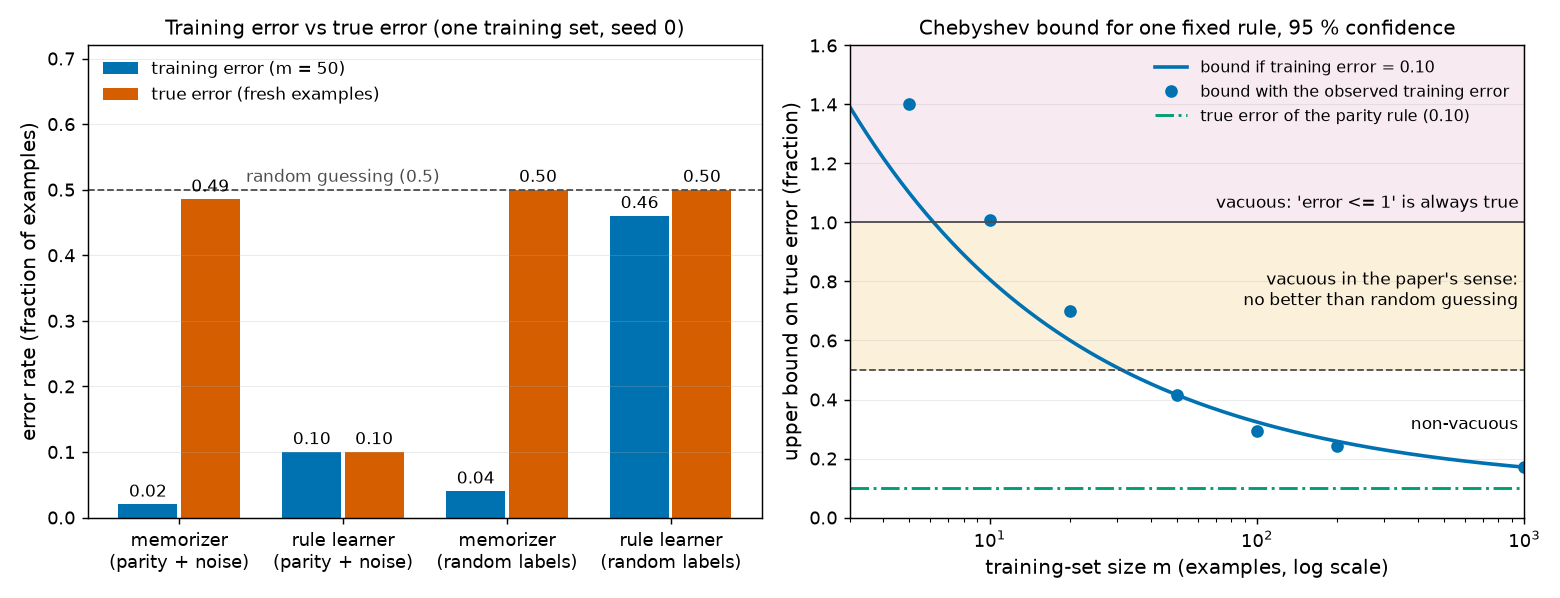
The left panel shows the lesson. A low training error is equally available with or without a real pattern. Only the true error separates the two worlds, and the true error is exactly what we cannot observe.
Many training sets¶
One training set could be a fluke, so the script repeats everything for 2,000 independent training sets.
| World | Learner | Mean training error | Mean true error | Mean gap | Smallest gap |
|---|---|---|---|---|---|
| parity + noise | memorizer | 0.0039 | 0.4844 | 0.4805 | 0.4304 |
| parity + noise | rule learner | 0.1014 | 0.1000 | −0.0014 | −0.1600 |
| random labels | memorizer | 0.0118 | 0.5000 | 0.4882 | 0.4400 |
| random labels | rule learner | 0.4209 | 0.5000 | 0.0791 | 0.0000 |
In the parity world the rule learner picked parity in every one of the 2,000 training sets (fraction 1.0000). Its gap averages almost zero, and is sometimes negative: on an unlucky training set, a good rule can look worse than it is.
The memorizer's gap never fell below 0.4304 in the parity world. Memorizing does not generalize, in any of the training sets.
A first real generalization bound¶
For one rule fixed before seeing any data, Chapter 1's Chebyshev inequality already gives a genuine generalization bound. With probability at least \(1-\delta\) over the draw of the training set,
Here \(m\) is the number of training examples and \(\delta\) the failure probability. The deeper block below derives it.
Take the parity rule, fixed in advance, and \(\delta = 0.05\). The gap term at \(m = 50\) is \(1/(2\sqrt{50 \times 0.05}) = 0.3162\). The training error of parity on our set is 0.100. So, with probability at least 0.95, the true error of the parity rule is below \(0.100 + 0.3162 = 0.4162\).
That bound is true (the actual true error is 0.1000). It is also non-vacuous in both senses: below 1, and below the random-guessing level 0.5.
The same calculation for other training-set sizes, using the first \(m\) examples of one long random sequence, gives:
| \(m\) | Gap term | Training error of parity | Bound | Verdict |
|---|---|---|---|---|
| 5 | 1.0000 | 0.400 | 1.4000 | vacuous: at least 1, says nothing |
| 10 | 0.7071 | 0.300 | 1.0071 | vacuous: at least 1 |
| 20 | 0.5000 | 0.200 | 0.7000 | vacuous in the paper's sense: no better than guessing |
| 50 | 0.3162 | 0.100 | 0.4162 | non-vacuous |
| 100 | 0.2236 | 0.070 | 0.2936 | non-vacuous |
| 200 | 0.1581 | 0.085 | 0.2431 | non-vacuous |
| 1000 | 0.0707 | 0.099 | 0.1697 | non-vacuous |
The right panel of the figure plots this. More data shrinks the gap term, and the bound walks down from "says nothing" through "true but no better than guessing" to "useful".
The same bound, misused¶
Now apply the identical formula to the memorizer. On the seed-0 set it would claim a true error below \(0.020 + 0.3162 = 0.3362\). The truth is 0.4852. The claim is false.
This is not bad luck. Over the 2,000 training sets, the claim was false in every one (fraction 1.0000). The formula assumed that the hypothesis was fixed before the data were drawn. The memorizer was built from the data, so the formula does not apply to it. Paying honestly for that choice is the subject of Chapters 10 and 11.
The paper's numbers¶
PAPER Table 1, p. 6; Table 2, p. 7 The paper reports bounds for GPT-2-style models and, in a "Random Guess" column, the levels a bound must beat. MY EXPLANATION Recomputing those levels with \(V = 50{,}257\):
| Quantity | Recomputed | Table 1 prints |
|---|---|---|
| Random-guess bits per token, \(\log_2 V\) | 15.6170 | 15.62 |
| Random-guess top-1 error, \(1 - 1/V\) | 99.9980 % | 99.99 |
| Random-guess top-10 error, \(1 - 10/V\) | 99.9801 % | 99.98 |
| Random-guess top-100 error, \(1 - 100/V\) | 99.8010 % | 99.80 |
Paper erratum E21: the top-1 random-guess level is truncated
PAPER Table 1, p. 6 The top-1 random-guess entry is printed as 99.99. MY EXPLANATION The exact value \(1 - 1/50{,}257 = 99.9980\,\%\) rounds to 100.00, not 99.99; the table truncates instead of rounding (erratum E21). No conclusion changes.
Classifying some of the paper's bounds against these levels (script output [8]):
| Table 1 entry | Bound | Random guess | Verdict |
|---|---|---|---|
| SubLoRA, top-1 error | 96.41 % | 99.9980 % | non-vacuous |
| Subspace Only, top-1 error | 96.52 % | 99.9980 % | non-vacuous |
| LoRA Only, top-1 error | 100 % | 99.9980 % | vacuous in both senses |
| Original Model, top-1 error | 100 % | 99.9980 % | vacuous in both senses |
| SubLoRA, bits per token | 12.12 | 15.6170 | non-vacuous |
| Original Model, bits per token | 70.76 | 15.6170 | vacuous |
Two lessons hide in this table. First, "non-vacuous" is a low bar: the best top-1 bound still allows the model's top guess to be wrong 96.41 % of the time. Second, a vacuous bound does not mean a bad model. PAPER Table 2, p. 7 The ordinary, uncompressed GPT-2 ("Original Model") scores 4.35 bits per token on held-out validation data (text kept aside from training, like a test set), far better than any compressed model, yet its bound of 70.76 says nothing. MY EXPLANATION The bound failed to certify it; the model did not fail to generalize.
Going deeper¶
Everything in this section is MY EXPLANATION unless tagged.
Two blocks sit next to the definitions they support: the expected risk of a trained hypothesis, and deterministic versus stochastic predictors. The four blocks below prove the toy bound, show exactly why it breaks for the memorizer, explain why random labels defeat a whole class of bounds, and pin down the two meanings of "vacuous".
Going deeper: a complete generalization bound for one fixed rule, proved from Chebyshev
Setting. Fix a hypothesis \(h\) before the training set is drawn. Use the 0-1 loss. Define \(Y_j = R(h, X_j) = \mathbf 1[h(z_j) \ne y_j]\) for \(j = 1, \dots, m\), and let \(p = R(h)\) be the unknown true error.
Step 1: the \(Y_j\) are i.i.d. Each \(Y_j\) is the same fixed function of \(X_j\). Functions applied separately to independent variables give independent variables, and identically distributed inputs give identically distributed outputs. So \(Y_1, \dots, Y_m\) are i.i.d. This step fails if \(h\) depends on the \(X_j\).
Step 2: mean and variance of one \(Y_j\). \(Y_j\) is 1 with probability \(p\) and 0 otherwise, so \(\mathbb E[Y_j] = p\). Because \(Y_j^2 = Y_j\) for a 0/1 variable, \(\mathbb E[Y_j^2] = p\) and
Step 3: the worst case. Completing the square, \(p(1-p) = \tfrac14 - \big(p - \tfrac12\big)^2 \le \tfrac14\), with equality only at \(p = \tfrac12\). We need this because \(p\) is unknown, and the gap term must be computable.
Step 4: the training error. \(\hat R(h) = \frac1m\sum_j Y_j\) is a sample mean. By linearity, \(\mathbb E[\hat R(h)] = p\). Because the \(Y_j\) are independent, their variances add (Chapter 1):
Step 5: Chebyshev. For any \(t > 0\),
Step 6: solve for \(t\). Setting \(1/(4mt^2) = \delta\) gives \(t = 1/(2\sqrt{m\delta})\). The event "\(p - \hat R(h) \ge t\)" is contained in "\(|\hat R(h) - p| \ge t\)", so it has probability at most \(\delta\). By the complement rule, with probability at least \(1-\delta\),
What is random, what is fixed. Random: the \(m\) training examples, hence \(\hat R(h)\). Fixed: \(h\), \(p\), \(m\), \(\delta\). Units: every quantity is a fraction of examples (an error rate).
Numbers. With \(m = 50\) and \(\delta = 0.05\): \(t = 0.3162\). For a training error of 0.10, the bound drops below 1 once \(m > 1/\big(4\delta(1 - 0.10)^2\big) = 6.17\), that is from \(m = 7\); it drops below the guessing level 0.5 once \(m > 1/\big(4\delta(0.5 - 0.10)^2\big) = 31.25\), that is from \(m = 32\) (output [4]). Both thresholds come from rearranging \(0.10 + 1/(2\sqrt{m\delta}) < c\) into \(m > 1/\big(4\delta(c - 0.10)^2\big)\).
How conservative is it? At \(m = 50\) the script computes the exact failure probability from the binomial distribution. For the parity rule (\(p = 0.1\)) the bound can never fail, because failure would need a training error below \(0.1 - 0.3162 < 0\). For the always 0 rule (\(p = 0.5\), the worst-case variance) failure needs at most 9 errors in 50; its probability is \(2.81 \times 10^{-6}\), far below the promised 0.05. Chebyshev uses only the variance and wastes most of its budget. Hoeffding's inequality (Chapter 9) uses the fact that each \(Y_j\) lies in \([0, 1]\) and shrinks the gap term at \(m = 50\) from 0.3162 to 0.1731.
Going deeper: why the bound breaks when training chooses h, and the price of choosing
What breaks. Step 1 of the previous proof needs \(h\) to be fixed before the data are drawn. For the memorizer, \(h = \hat h_S\) is built so that \(R(\hat h_S, X_j)\) is 0 for almost every training example. These losses are not independent draws whose mean is \(R(\hat h_S)\); their mean is close to 0 by construction. Plugging them into the fixed-\(h\) formula produced a claim that was false in all 2,000 training sets (output [5]); the smallest true gap, 0.4304, exceeded the claimed margin 0.3162 every time.
The repair for finitely many candidates. Suppose training can only output one of \(N\) hypotheses \(h_1, \dots, h_N\), all fixed in advance. Give each a failure budget \(\delta/N\). Let \(A_i\) be the event "the bound for \(h_i\) fails". The union bound (Chapter 10 proves it) says that the probability that at least one of several events happens is at most the sum of their probabilities:
So with probability at least \(1-\delta\), every candidate satisfies its bound at once, including whichever one training picks. The price is a larger gap term, because each bound is computed with \(\delta/N\) in place of \(\delta\).
The price in numbers (\(m = 50\), \(\delta = 0.05\), output [5]):
| Candidates \(N\) | Tool | Gap term | Bound |
|---|---|---|---|
| 4 rules | Chebyshev, \(1/(2\sqrt{m\delta/N})\) | 0.6325 | rule learner: 0.100 + 0.6325 = 0.7325 |
| 1 (fixed rule) | Hoeffding, Chapter 9 | 0.1731 | parity rule: 0.100 + 0.1731 = 0.2731 |
| 4 rules | Hoeffding, Chapter 9 | 0.2093 | rule learner: 0.100 + 0.2093 = 0.3093 |
| \(2^{1000}\) lookup tables | Hoeffding, Chapter 9 | 2.6385 | memorizer: 0.020 + 2.6385 = 2.6585 |
The Hoeffding rows use the gap term \(\sqrt{(\ln N + \ln(1/\delta))/(2m)}\), which Chapter 10 derives. Chebyshev's version pays heavily even for 4 candidates (vacuous in the paper's sense); Hoeffding's pays little. But even Hoeffding cannot afford \(2^{1000}\) candidates: the memorizer's bound exceeds 1.
The seed of the paper's idea. In the Hoeffding gap term, \(\ln N = (\log_2 N) \ln 2\), and \(\log_2 N\) is the number of yes/no answers needed to name one candidate: 0 for a fixed rule, 2 for one of four rules, 1000 for one lookup table. A hypothesis that can be named with few yes/no answers is cheap to certify. Chapters 11 to 14 turn this into the paper's compression bound, where the "name" of a model is its compressed file.
Going deeper: random labels defeat any bound that looks only at the hypothesis space
PAPER §2, p. 3 The paper recalls that classical bounds, built on complexity measures of the hypothesis space as a whole (VC dimension, Rademacher complexity), were vacuous for neural networks, because networks are flexible enough to fit randomly labelled training data (Zhang et al., 2021). MY EXPLANATION The toy lets us prove this in miniature.
Claim. Let \(\mathcal H_{\text{all}}\) be all \(2^{1000}\) lookup tables, \(m = 50\) and \(\delta = 0.05\). Suppose a number \(\varepsilon\), depending only on \((\mathcal H_{\text{all}}, m, \delta)\), has this property: for every data-generating process on inputs \(\{0, \dots, 999\}\), with probability at least \(1-\delta\), every \(h \in \mathcal H_{\text{all}}\) satisfies \(R(h) \le \hat R(h) + \varepsilon\). Then \(\varepsilon \ge 0.5\).
Proof. Use the random-label process. There, every \(h\) has \(R(h) = 0.5\), because the label is a fair coin independent of \(z\), so any fixed answer is wrong with probability \(\tfrac12\).
Let \(E\) be the event "the 50 training inputs are all distinct". Drawing them one by one, the \(j\)-th draw must avoid the \(j-1\) inputs already drawn, so
(output [6]). On \(E\), the lookup table \(h_S\) that answers each training input with its training label (and, say, 0 elsewhere) has \(\hat R(h_S) = 0\).
Let \(G\) be the event "the bound holds for every \(h\)"; by assumption \(\Pr(G) \ge 0.95\). Since \(\Pr(E \text{ or } G) \le 1\),
So at least one training set lies in both events. For it, \(0.5 = R(h_S) \le \hat R(h_S) + \varepsilon = \varepsilon\). Hence \(\varepsilon \ge 0.5\). (The script's simulation finds the memorizer's training error is exactly 0 in a fraction 0.5450 of random-label training sets — more than \(\Pr(E)\), because repeated inputs with equal labels also fit.)
Consequence. The same \(\varepsilon\) must be used in the parity world, because it depends only on \((\mathcal H_{\text{all}}, m, \delta)\). There the parity rule, which belongs to \(\mathcal H_{\text{all}}\), would get a bound of at least \(0.10 + 0.5 = 0.6\): vacuous in the paper's sense, even though parity is an excellent rule.
The escape. Let the gap term depend on which hypothesis was chosen. A weighting of hypotheses fixed before the data (the prior \(P(h)\) of Chapter 11) can give simple rules a small gap term and arbitrary lookup tables a huge one. PAPER §2, p. 3; §4.1, p. 4 This is the move the paper borrows from PAC-Bayes and compression bounds: complexity is measured for the found model, not for the whole space.
Going deeper: the two meanings of vacuous, made exact
Standard meaning. For a loss that always lies in \([a, b]\), the statement \(R(h) \le b\) is true for every hypothesis and every data-generating process, without any data. A bound \(R(\hat h) \le B\) is vacuous in the standard sense when \(B \ge b\). For an error rate, \(b = 1\) (100 %).
PAPER §1, p. 2; §6.2, p. 7 The paper's meaning. A bound is vacuous when \(B\) is at least the risk of random guessing.
MY EXPLANATION The two random-guess levels come from these calculations.
- Top-k error. Rank the \(V\) tokens in a uniformly random order. The actual next token is equally likely to be at any of the \(V\) positions, so it lands in the top \(k\) with probability \(k/V\). The expected error is \(1 - k/V\), whatever the text.
- Bits per token. Give every token probability \(1/V\). The model's surprise at the actual token, measured in bits, is \(\log_2\big(1/(1/V)\big) = \log_2 V\) (Chapter 3 and Chapter 6 define this measure). It is the same for every token of every document, so the average is \(\log_2 V = 15.6170\) bits per token for \(V = 50{,}257\).
Why the stricter bar. A bound between the guessing level and the always-true level is true but certifies nothing about learning: a model that knew nothing would satisfy it. Beating the guessing level certifies that the model is better than knowing nothing. For bits per token there is a further reason: an ordinary language model's loss has no upper limit (a token given probability 0 costs infinitely many bits), so the standard meaning has nothing to compare with. Chapter 16 shows how the paper caps the loss.
In the toy. With two labels, guessing has error 0.5 and the always-true level is 1. The \(m = 20\) bound 0.7000 is vacuous in the paper's sense but not in the standard sense; the \(m = 10\) bound 1.0071 is vacuous in both.
Common misconceptions¶
- Misconception: "A model with near-zero training error has learned the task." — Actually: the memorizer has training error 0.020 and true error 0.4852. With random labels, where there is nothing to learn, its training error is still only 0.040.
- Misconception: "A vacuous bound means the model generalizes badly." — Actually: a bound is only an upper limit. The paper's uncompressed GPT-2 has a vacuous bound of 70.76 bits per token but a validation score of 4.35 bits per token, the best in the paper. The bound failed to certify the model; the model did not fail.
- Misconception: "A non-vacuous bound proves the model does not memorize." — Actually: a bound limits the expected risk on fresh examples. A model can memorize some training text verbatim and still have a low expected risk. Whether the paper's results speak to memorization is examined in Chapter 29.
- Misconception: "A generalization bound is a fancier way of measuring test error." — Actually: a test set measures one finished hypothesis directly, and usually more tightly. A bound uses only training data plus a description of the hypothesis. Its value is explanatory: it shows that generalization follows from low training error and simplicity.
- Misconception: "The generalization gap is always positive." — Actually: for a rule fixed in advance the average gap is zero (−0.0014 over 2,000 training sets for the rule learner), and on an unlucky training set it is negative (as low as −0.1600).
- Misconception: "A model that outputs probabilities is a stochastic predictor." — Actually: the same input always produces the same probabilities, so it is one deterministic function. "Stochastic" refers to randomness in which hypothesis is used, as with the coin-flipping memorizer.
Self-test¶
Q1. A rule was fixed before any data were collected. On \(m = 200\) training examples it has training error 0.12. Using the Chebyshev bound of this chapter with \(\delta = 0.05\), what upper bound do you get on its true error? Is the bound vacuous in the standard sense, vacuous in the paper's sense (for a two-label task), or non-vacuous?
Answer
The gap term is \(1/(2\sqrt{m\delta}) = 1/(2\sqrt{200 \times 0.05}) = 1/(2\sqrt{10}) = 0.1581\). The bound is \(0.12 + 0.1581 = 0.2781\) (output [Q1]). It is below 1 and below the guessing level 0.5, so it is non-vacuous in both senses.
What it means: with probability at least 0.95 over the random draw of the 200 training examples, the rule's true error is below 0.2781. It is valid only because the rule was fixed before the data were seen.
Q2. A colleague trains a lookup table on 50 examples, finds training error 0.020, and reports: "By Chebyshev, with 95 % confidence, the true error is below \(0.020 + 0.3162 = 0.3362\)." What is wrong, and what would an honest bound look like?
Answer
The formula assumes the hypothesis was fixed before the training set was drawn. Then its training losses are i.i.d. with mean equal to the true error. The lookup table was built from the training set, so its training losses are near 0 by construction and say nothing about fresh examples. In the toy, the colleague's kind of claim was false in all 2,000 training sets; for the seed-0 set the true error is 0.4852.
An honest bound must pay for the choice among all the hypotheses training could have produced. For \(2^{1000}\) lookup tables, even Hoeffding's inequality with the union bound gives a gap term of 2.6385, so the bound (\(0.020 + 2.6385 = 2.6585\)) is vacuous. That is the correct verdict: nothing about the table's training error certifies its performance on new inputs.
Q3. Classify each of these bounds from the paper's Table 1 as vacuous in the standard sense, vacuous only in the paper's sense, or non-vacuous: (a) LoRA Only, top-1 error 100 %; (b) Subspace Only, top-1 error 96.52 %; (c) Original Model, 70.76 bits per token; (d) SubLoRA, 12.12 bits per token. What does (b) tell you about how accurate that model is?
Answer
(a) Vacuous in the standard sense: an error rate is always at most 100 %, so the bound says nothing. It is also above the guessing level 99.9980 %.
(b) Non-vacuous: 96.52 % is below the guessing level 99.9980 %. But it only certifies that the model's top guess is wrong at most 96.52 % of the time on fresh documents (with probability at least 0.95 over the training data). That is better than guessing, yet far from accurate.
(c) Vacuous in the paper's sense: 70.76 is above \(\log_2 50{,}257 = 15.6170\) bits per token. There is no standard always-true level to compare with, because this loss has no upper limit for an ordinary model.
(d) Non-vacuous: 12.12 is below 15.6170.
Code for this chapter¶
Run it from the project root:
.venv/Scripts/python explainer/code/ch02_memorizer.py
Source: ch02_memorizer.py
"""Chapter 2 demo: a memorizer vs a simple rule on a toy task, and what a generalization bound is.

Claims reproduced / illustrated (all [MY EXPLANATION] unless tagged):
  [1] Toy task: input z uniform on {0,...,999}; label y = parity of z, flipped with probability 0.1.
      One training set of m = 50 pairs (seed 0). Memorizer = lookup table, fair coin on unseen inputs.
      Rule learner = the best of 4 rules {parity, anti-parity, always 0, always 1} on the training set.
      Training error, exact true error (we know the process) and an estimate on 200,000 fresh draws.
  [2] Random-labels variant (same inputs, labels are fair coin flips): the memorizer still fits the
      training set; every predictor has true error exactly 0.5.
  [3] Averages over 2,000 independent training sets in both worlds.
  [4] A genuine generalization bound for ONE rule fixed in advance, from Chebyshev (Chapter 1):
      R(h) < Rhat(h) + 1/(2 sqrt(m delta)) with probability >= 1 - delta. Vacuous vs non-vacuous as m grows;
      exact failure probabilities (binomial).
  [5] Applying that fixed-rule bound to the memorizer fails in every training set; the price of choosing
      among N hypotheses (preview of Chapters 9-11, using pacbound.hoeffding_t).
  [6] Random labels defeat any bound whose gap depends only on the hypothesis space (Zhang et al. argument
      in miniature): Pr(all 50 training inputs distinct) is computed exactly.
  [7] Stochastic vs deterministic predictors: the coin-flipping memorizer vs 10,000 "frozen" memorizers.
  [8] The paper's random-guess levels log2 V and 1 - k/V [PAPER §1 p. 2, §6.2 p. 7] vs Table 1's
      "Random Guess" column, and the vacuous / non-vacuous status of some Table 1-2 entries.
  [Q1] Numbers for the chapter's self-test.

Writes outputs/ch02_memorizer.txt and docs/assets/fig/ch02_train_vs_true.png. Runtime: a few seconds.
"""
import math
import sys
from pathlib import Path

import numpy as np
from scipy.stats import binom

HERE = Path(__file__).resolve().parent
sys.path.insert(0, str(HERE))
import pacbound  # noqa: E402

import matplotlib  # noqa: E402
matplotlib.use("Agg")
import matplotlib.pyplot as plt  # noqa: E402

OUT_TXT = HERE / "outputs" / "ch02_memorizer.txt"
OUT_FIG = HERE.parent / "docs" / "assets" / "fig" / "ch02_train_vs_true.png"
OUT_TXT.parent.mkdir(parents=True, exist_ok=True)
OUT_FIG.parent.mkdir(parents=True, exist_ok=True)

N_INPUTS = 1000          # inputs z = 0..999, each with probability 1/1000
NOISE = 0.1              # probability that the parity label is flipped
M = 50                   # training-set size m
N_FRESH = 200_000        # fresh draws used to estimate the true error
REPS = 2_000             # independent training sets for the averages in [3] and [5]
N_FROZEN = 10_000        # frozen memorizers in [7]
DELTA = pacbound.DELTA   # 0.05: our choice for the toy; same value as the authors' code [SOURCE, erratum E31]
RULES = ["parity", "anti-parity", "always 0", "always 1"]
ZS = np.arange(N_INPUTS)
RULE_PRED = np.stack([ZS % 2, 1 - ZS % 2, np.zeros_like(ZS), np.ones_like(ZS)])  # shape (4, 1000)
rng = np.random.default_rng(0)
lines = []


def out(s=""):
    lines.append(s)


def p_label1(world):
    """Pr(y = 1 | z) for every z. Structured world: 0.9 for odd z, 0.1 for even z. Random world: 0.5."""
    if world == "structured":
        return np.where(ZS % 2 == 1, 1.0 - NOISE, NOISE)
    return np.full(N_INPUTS, 0.5)


def draw_labels(world, z, rng):
    return (rng.random(z.shape) < p_label1(world)[z]).astype(np.int64)


def err_table(world):
    """err[c, z] = Pr(y != c | z): probability that answering c on input z is wrong (c = 0 or 1)."""
    p1 = p_label1(world)
    return np.stack([p1, 1.0 - p1])


def true_risk_det(pred, world):
    """Exact expected 0-1 risk of a deterministic predictor given as an array pred[z] over all z."""
    return float(err_table(world)[pred, ZS].mean())


def fit_memorizer(z, y):
    """Lookup table: for each seen z, the majority label among its copies (ties -> label seen first);
    -1 marks an unseen input (the memorizer will flip a fair coin there)."""
    c = np.bincount(z, minlength=N_INPUTS)
    c1 = np.bincount(z, weights=y, minlength=N_INPUTS).astype(np.int64)
    c0 = c - c1
    stored = np.full(N_INPUTS, -1)
    seen = c > 0
    stored[seen & (c1 > c0)] = 1
    stored[seen & (c0 > c1)] = 0
    ties = seen & (c1 == c0)
    if ties.any():
        uz, first = np.unique(z, return_index=True)
        first_label = np.full(N_INPUTS, -1)
        first_label[uz] = y[first]
        stored[ties] = first_label[ties]
    return stored


def mem_true_risk(stored, world):
    """Exact expected risk of the coin-flipping memorizer (expectation over the fresh example AND the coin):
    an unseen input is answered correctly with probability 1/2 whatever its label."""
    err = np.full(N_INPUTS, 0.5)
    seen = stored >= 0
    err[seen] = err_table(world)[stored[seen], ZS[seen]]
    return float(err.mean())


def fit_rules(z, y):
    """Training error of each of the 4 rules; argmin keeps the first rule on ties (list order)."""
    errs = (RULE_PRED[:, z] != y).mean(axis=1)
    return int(np.argmin(errs)), errs


def cheb_gap(m, delta=DELTA, n_hyp=1):
    """Chebyshev gap for a 0-1 loss (variance <= 1/4): 1/(2 sqrt(m delta / n_hyp)). Fraction (error rate)."""
    return 1.0 / (2.0 * math.sqrt(m * delta / n_hyp))


# ------------------------------------------------------------------ data
Z_ALL = rng.integers(0, N_INPUTS, size=1000)          # one long i.i.d. sequence of inputs
Y_ALL = draw_labels("structured", Z_ALL, rng)
z_tr, y_tr = Z_ALL[:M], Y_ALL[:M]                      # the training set = its first m = 50 pairs
y_rand = rng.integers(0, 2, size=M)                    # random-labels world: same inputs, coin-flip labels
n_distinct = len(np.unique(z_tr))

out("Chapter 2 demo (seed 0). Toy task: z uniform on {0..999}; y = parity(z) flipped w.p. 0.1; 0-1 loss")
out(f"[1]-[2] One training set, m = {M}: {n_distinct} distinct inputs ({M - n_distinct} repeats).")
uz, cnt = np.unique(z_tr, return_counts=True)
for zz in uz[cnt > 1]:
    out(f"    input z = {zz} appears {int(np.sum(z_tr == zz))} times; labels (parity world) "
        f"{list(map(int, y_tr[z_tr == zz]))}, (random world) {list(map(int, y_rand[z_tr == zz]))}")
out(f"    true error = exact (we know the process); fresh = estimate on {N_FRESH:,} new draws")
out("  world            learner (chosen rule)      train err  true err  fresh est. (+-1 s.e.)   gap")
results = {}
for world, y in [("structured", y_tr), ("random", y_rand)]:
    stored = fit_memorizer(z_tr, y)
    k, rule_errs = fit_rules(z_tr, y)
    zf = rng.integers(0, N_INPUTS, size=N_FRESH)
    yf = draw_labels(world, zf, rng)
    pm = stored[zf].copy()
    unseen = pm < 0
    pm[unseen] = rng.integers(0, 2, size=int(unseen.sum()))           # fresh coin for each unseen query
    rows = [("memorizer", float(np.mean(stored[z_tr] != y)), mem_true_risk(stored, world),
             float(np.mean(pm != yf))),
            (f"rule learner ({RULES[k]})", float(rule_errs[k]), true_risk_det(RULE_PRED[k], world),
             float(np.mean(RULE_PRED[k, zf] != yf)))]
    label = "parity+10% noise" if world == "structured" else "random labels"
    for name, tr, tru, est in rows:
        se = math.sqrt(tru * (1 - tru) / N_FRESH)
        assert abs(est - tru) < 5 * se
        out(f"  {label:16s} {name:26s} {tr:8.3f}  {tru:8.4f}   {est:.4f} (+-{se:.4f})  {tru - tr:6.3f}")
        results[(world, name.split(" (")[0])] = (tr, tru)
    if world == "structured":
        seen = stored >= 0
        good = int(np.sum(stored[seen] == ZS[seen] % 2))
        bad = int(seen.sum()) - good
        n_unseen = N_INPUTS - int(seen.sum())
        decomp = (n_unseen * 0.5 + good * NOISE + bad * (1 - NOISE)) / N_INPUTS
        assert abs(decomp - rows[0][2]) < 1e-12
        out(f"    memorizer true error = ({n_unseen} unseen x 0.5 + {good} stored-correct x 0.1 + "
            f"{bad} stored-flipped x 0.9)/1000 = {decomp:.4f}")
        out("    training errors of the 4 rules: " +
            ", ".join(f"{r} {e:.2f}" for r, e in zip(RULES, rule_errs)))
        out("    true errors of the 4 rules:     " +
            ", ".join(f"{r} {true_risk_det(RULE_PRED[j], world):.2f}" for j, r in enumerate(RULES)))
        stored_struct = stored

# ------------------------------------------------- [3] many training sets
out(f"[3] Averages over {REPS:,} independent training sets (m = {M} each)")
out("  world            learner         mean train  mean true  mean gap  min gap")
mem_gaps_struct = None
for world in ["structured", "random"]:
    acc = {"memorizer": [], "rule learner": []}
    picked_parity = 0
    for _ in range(REPS):
        z = rng.integers(0, N_INPUTS, size=M)
        y = draw_labels(world, z, rng)
        st = fit_memorizer(z, y)
        acc["memorizer"].append((float(np.mean(st[z] != y)), mem_true_risk(st, world)))
        k, errs = fit_rules(z, y)
        picked_parity += (k == 0)
        acc["rule learner"].append((float(errs[k]), true_risk_det(RULE_PRED[k], world)))
    label = "parity+10% noise" if world == "structured" else "random labels"
    for name, vals in acc.items():
        a = np.array(vals)
        gaps = a[:, 1] - a[:, 0]
        out(f"  {label:16s} {name:14s} {a[:, 0].mean():9.4f}  {a[:, 1].mean():9.4f}  {gaps.mean():8.4f} "
            f" {gaps.min():7.4f}")
        if world == "structured" and name == "memorizer":
            mem_gaps_struct = gaps
        if world == "random" and name == "memorizer":
            frac_zero_random = float(np.mean(a[:, 0] == 0))
    if world == "structured":
        out(f"    rule learner picked 'parity' in {picked_parity / REPS:.4f} of the training sets")

# ------------------------------------- [4] Chebyshev bound for one fixed rule
t50 = cheb_gap(M)
out(f"[4] Fixed rule 'parity' (chosen BEFORE seeing data). Chebyshev: R(h) < Rhat(h) + 1/(2 sqrt(m delta)) "
    f"w.p. >= {1 - DELTA:.2f}")
out("     m    gap t   Rhat(parity)  bound    verdict (0-1 loss: always-true level 1, guessing 0.5)")
for m in [5, 10, 20, 50, 100, 200, 1000]:
    t = cheb_gap(m)
    rh = float(np.mean(RULE_PRED[0, Z_ALL[:m]] != Y_ALL[:m]))       # prefix of the same i.i.d. sequence
    b = rh + t
    verdict = ("vacuous (>= 1, says nothing)" if b >= 1 else
               "vacuous in the paper's sense (>= 0.5)" if b >= 0.5 else "non-vacuous")
    out(f"  {m:5d}   {t:.4f}    {rh:.3f}       {b:.4f}   {verdict}")
for level, name in [(1.0, "below 1 (standard non-vacuous)"), (0.5, "below 0.5 (beats random guessing)")]:
    m_need = 1.0 / (4.0 * DELTA * (level - NOISE) ** 2)        # solve 0.1 + 1/(2 sqrt(m delta)) < level
    out(f"    with Rhat = {NOISE:.2f}: bound {name} once m > {m_need:.2f}, i.e. m >= {math.floor(m_need) + 1}")
for p, nm in [(NOISE, "parity (true error 0.1)"), (0.5, "always 0 (true error 0.5)")]:
    kmax = math.floor(M * (p - t50) + 1e-12)
    pf = float(binom.cdf(kmax, M, p)) if kmax >= 0 else 0.0
    assert pf <= DELTA
    out(f"    exact Pr(bound fails) at m = {M} for rule {nm}: {pf:.2e}  (guaranteed <= {DELTA})")
t_hoef = pacbound.hoeffding_t(M, 1.0, math.log(1.0 / DELTA))
out(f"    preview: Hoeffding (Chapter 9) shrinks the gap at m = {M} from {t50:.4f} to {t_hoef:.4f}")

# -------------------------------- [5] misuse on the memorizer; price of choice
fails = float(np.mean(mem_gaps_struct >= t50))
mem_tr0, mem_true0 = results[("structured", "memorizer")]
rl_tr0 = results[("structured", "rule learner")][0]
out(f"[5] Misuse on the memorizer (chosen AFTER seeing the data): 'true < train + {t50:.4f}'; seed 0: "
    f"{mem_tr0:.3f} + {t50:.4f} = {mem_tr0 + t50:.4f} vs true {mem_true0:.4f}")
out(f"    is false in {fails:.4f} of the {REPS:,} training sets of [3] (parity world)")
out("    price of choosing among N hypotheses, m = 50, delta = 0.05 (union bound, Chapters 10-11):")
g4c = cheb_gap(M, n_hyp=4)
out(f"      Chebyshev, N = 4 rules          : gap {g4c:.4f} -> rule learner {rl_tr0:.3f} + {g4c:.4f} = "
    f"{rl_tr0 + g4c:.4f}")
for n_hyp_log2, nm, who, tr in [(0, "N = 1 (fixed rule)", "parity rule", rl_tr0),
                                (2, "N = 4 rules", "rule learner", rl_tr0),
                                (1000, "N = 2^1000 tables", "memorizer", mem_tr0)]:
    g = pacbound.hoeffding_t(M, 1.0, n_hyp_log2 * math.log(2) + math.log(1.0 / DELTA))
    out(f"      Hoeffding, {nm:21s}: gap {g:.4f} -> {who} {tr:.3f} + {g:.4f} = {tr + g:.4f}  "
        f"(log2 N = {n_hyp_log2})")

# ------------------------------------------------------ [6] random labels
p_distinct = math.prod(1 - j / N_INPUTS for j in range(M))
assert p_distinct > DELTA
out(f"[6] Random labels: Pr(all {M} training inputs distinct) = {p_distinct:.4f} (exact; then train err = 0)")
out(f"    simulated Pr(memorizer train err = 0) = {frac_zero_random:.4f}; both > delta = {DELTA}; "
    f"Pr(E and G) >= {p_distinct:.4f} + {1 - DELTA:.2f} - 1 = {p_distinct + (1 - DELTA) - 1:.4f} > 0")

# ------------------------------------------- [7] stochastic vs deterministic
risk_avg = mem_true_risk(stored_struct, "structured")
coins = rng.integers(0, 2, size=(N_FROZEN, N_INPUTS))
frozen_pred = np.where(stored_struct >= 0, stored_struct, coins)       # each row = one frozen memorizer
frozen_risk = err_table("structured")[frozen_pred, ZS].mean(axis=1)
assert abs(frozen_risk.mean() - risk_avg) < 0.001
out(f"[7] Coin-flipping (stochastic) memorizer from [1]: true error {risk_avg:.4f} = average over its coins.")
out(f"    {N_FROZEN:,} frozen (deterministic) versions: mean {frozen_risk.mean():.4f}, "
    f"sd {frozen_risk.std():.4f}, min {frozen_risk.min():.4f}, max {frozen_risk.max():.4f}")

# ---------------------------------------------- [8] the paper's baselines
V = pacbound.V_GPT2
bpd_rg = pacbound.random_guess_bpd(V)
assert round(bpd_rg, 2) == 15.62
out(f"[8] Paper: V = {V:,}. Random-guess BPD log2 V = {bpd_rg:.4f} bits/token (Table 1: 15.62, "
    f"diff {bpd_rg - 15.62:+.4f})")
for k, tab in [(1, 99.99), (10, 99.98), (100, 99.80)]:
    e = 100 * pacbound.random_guess_topk_error(k, V)
    assert math.floor(e * 100) / 100 == tab          # Table 1 truncates (erratum E21)
    note = "  -> rounds to 100.00; table truncates (E21)" if round(e, 2) != tab else ""
    out(f"    top-{k:<3d} error 1 - k/V = {e:.4f} %  (Table 1: {tab:.2f}){note}")
rg1 = 100 * pacbound.random_guess_topk_error(1, V)
paper = [("Table 1 SubLoRA top-1 error", 96.41, rg1, "%"),
         ("Table 1 Subspace Only top-1 error", 96.52, rg1, "%"),
         ("Table 1 LoRA Only top-1 error", 100.0, rg1, "%"),
         ("Table 1 Original Model top-1 error", 100.0, rg1, "%"),
         ("Table 1 SubLoRA BPD", 12.12, bpd_rg, "bits/token"),
         ("Table 1 Original Model BPD", 70.76, bpd_rg, "bits/token")]
for nm, b, rg, unit in paper:
    status = "non-vacuous" if b < rg else ("vacuous (= 100 %, always true)" if b >= 100 else "vacuous")
    out(f"    {nm:35s} {b:6.2f} {unit:10s} vs random guess {rg:.3f}: {status}")
out("      (Original Model validation BPD, Table 2: 4.35 bits/token -- a good model with a vacuous bound)")
out(f"    paper scale: m = {pacbound.M_DOCS:,} documents [SOURCE nanoGPT, E32]; GPT-2 small "
    f"{pacbound.gpt2_params(12, 768):,} params (paper: 124M)")

# ---------------------------------------------------------- self-test Q1
tq = cheb_gap(200)
out(f"[Q1] m = 200, delta = 0.05, Rhat = 0.12: gap 1/(2 sqrt(200*0.05)) = {tq:.4f}; bound = {0.12 + tq:.4f}")

# ------------------------------------------------------------------ figure
fig, (ax1, ax2) = plt.subplots(1, 2, figsize=(12, 4.6))
groups = [("structured", "memorizer"), ("structured", "rule learner"),
          ("random", "memorizer"), ("random", "rule learner")]
names = ["memorizer\n(parity + noise)", "rule learner\n(parity + noise)",
         "memorizer\n(random labels)", "rule learner\n(random labels)"]
xs = np.arange(len(groups))
tr = [results[g][0] for g in groups]
tu = [results[g][1] for g in groups]
ax1.bar(xs - 0.19, tr, width=0.36, color="#0072B2", label="training error (m = 50)")
ax1.bar(xs + 0.19, tu, width=0.36, color="#D55E00", label="true error (fresh examples)")
for x, a, b in zip(xs, tr, tu):
    ax1.text(x - 0.19, a + 0.012, f"{a:.2f}", ha="center", fontsize=9.5)
    ax1.text(x + 0.19, b + 0.012, f"{b:.2f}", ha="center", fontsize=9.5)
ax1.axhline(0.5, color="0.3", lw=1.0, ls="--")
ax1.text(1.0, 0.512, "random guessing (0.5)", ha="center", fontsize=9.5, color="0.3")
ax1.set_xticks(xs)
ax1.set_xticklabels(names, fontsize=9.5)
ax1.set_ylim(0, 0.72)
ax1.set_ylabel("error rate (fraction of examples)", fontsize=11)
ax1.set_title("Training error vs true error (one training set, seed 0)", fontsize=11)
ax1.legend(fontsize=9.5, frameon=False, loc="upper left")

mgrid = np.logspace(math.log10(3), 3, 400)
ax2.axhspan(1.0, 1.6, color="#CC79A7", alpha=0.15)
ax2.axhspan(0.5, 1.0, color="#E69F00", alpha=0.15)
ax2.plot(mgrid, NOISE + 1 / (2 * np.sqrt(mgrid * DELTA)), color="#0072B2", lw=2,
         label="bound if training error = 0.10")
ms = np.array([5, 10, 20, 50, 100, 200, 1000])
rh = np.array([np.mean(RULE_PRED[0, Z_ALL[:m]] != Y_ALL[:m]) for m in ms])
ax2.plot(ms, rh + 1 / (2 * np.sqrt(ms * DELTA)), "o", color="#0072B2", ms=6,
         label="bound with the observed training error")
ax2.axhline(NOISE, color="#009E73", lw=1.6, ls="-.", label="true error of the parity rule (0.10)")
ax2.axhline(1.0, color="0.3", lw=1.0)
ax2.axhline(0.5, color="0.3", lw=1.0, ls="--")
ax2.text(950, 1.05, "vacuous: 'error <= 1' is always true", ha="right", fontsize=9.5)
ax2.text(950, 0.72, "vacuous in the paper's sense:\nno better than random guessing", ha="right", fontsize=9.5)
ax2.text(950, 0.30, "non-vacuous", ha="right", fontsize=9.5)
ax2.set_xscale("log")
ax2.set_xlim(3, 1000)
ax2.set_ylim(0, 1.6)
ax2.set_xlabel("training-set size m (examples, log scale)", fontsize=11)
ax2.set_ylabel("upper bound on true error (fraction)", fontsize=11)
ax2.set_title("Chebyshev bound for one fixed rule, 95 % confidence", fontsize=11)
ax2.legend(fontsize=9, frameon=False, loc="upper right")
for ax in (ax1, ax2):
    ax.tick_params(labelsize=10)
    ax.grid(alpha=0.25, lw=0.6, axis="y")
fig.tight_layout()
fig.savefig(OUT_FIG, dpi=130)
out(f"figure: docs/assets/fig/{OUT_FIG.name}")

text = "\n".join(lines) + "\n"
print(text, end="")
OUT_TXT.write_text(text, encoding="utf-8")
Output:
Chapter 2 demo (seed 0). Toy task: z uniform on {0..999}; y = parity(z) flipped w.p. 0.1; 0-1 loss
[1]-[2] One training set, m = 50: 47 distinct inputs (3 repeats).
    input z = 175 appears 2 times; labels (parity world) [1, 1], (random world) [0, 1]
    input z = 670 appears 2 times; labels (parity world) [0, 0], (random world) [0, 0]
    input z = 729 appears 2 times; labels (parity world) [0, 1], (random world) [0, 1]
    true error = exact (we know the process); fresh = estimate on 200,000 new draws
  world            learner (chosen rule)      train err  true err  fresh est. (+-1 s.e.)   gap
  parity+10% noise memorizer                     0.020    0.4852   0.4826 (+-0.0011)   0.465
  parity+10% noise rule learner (parity)         0.100    0.1000   0.0995 (+-0.0007)   0.000
    memorizer true error = (953 unseen x 0.5 + 42 stored-correct x 0.1 + 5 stored-flipped x 0.9)/1000 = 0.4852
    training errors of the 4 rules: parity 0.10, anti-parity 0.90, always 0 0.56, always 1 0.44
    true errors of the 4 rules:     parity 0.10, anti-parity 0.90, always 0 0.50, always 1 0.50
  random labels    memorizer                     0.040    0.5000   0.5009 (+-0.0011)   0.460
  random labels    rule learner (anti-parity)    0.460    0.5000   0.4992 (+-0.0011)   0.040
[3] Averages over 2,000 independent training sets (m = 50 each)
  world            learner         mean train  mean true  mean gap  min gap
  parity+10% noise memorizer         0.0039     0.4844    0.4805   0.4304
  parity+10% noise rule learner      0.1014     0.1000   -0.0014  -0.1600
    rule learner picked 'parity' in 1.0000 of the training sets
  random labels    memorizer         0.0118     0.5000    0.4882   0.4400
  random labels    rule learner      0.4209     0.5000    0.0791   0.0000
[4] Fixed rule 'parity' (chosen BEFORE seeing data). Chebyshev: R(h) < Rhat(h) + 1/(2 sqrt(m delta)) w.p. >= 0.95
     m    gap t   Rhat(parity)  bound    verdict (0-1 loss: always-true level 1, guessing 0.5)
      5   1.0000    0.400       1.4000   vacuous (>= 1, says nothing)
     10   0.7071    0.300       1.0071   vacuous (>= 1, says nothing)
     20   0.5000    0.200       0.7000   vacuous in the paper's sense (>= 0.5)
     50   0.3162    0.100       0.4162   non-vacuous
    100   0.2236    0.070       0.2936   non-vacuous
    200   0.1581    0.085       0.2431   non-vacuous
   1000   0.0707    0.099       0.1697   non-vacuous
    with Rhat = 0.10: bound below 1 (standard non-vacuous) once m > 6.17, i.e. m >= 7
    with Rhat = 0.10: bound below 0.5 (beats random guessing) once m > 31.25, i.e. m >= 32
    exact Pr(bound fails) at m = 50 for rule parity (true error 0.1): 0.00e+00  (guaranteed <= 0.05)
    exact Pr(bound fails) at m = 50 for rule always 0 (true error 0.5): 2.81e-06  (guaranteed <= 0.05)
    preview: Hoeffding (Chapter 9) shrinks the gap at m = 50 from 0.3162 to 0.1731
[5] Misuse on the memorizer (chosen AFTER seeing the data): 'true < train + 0.3162'; seed 0: 0.020 + 0.3162 = 0.3362 vs true 0.4852
    is false in 1.0000 of the 2,000 training sets of [3] (parity world)
    price of choosing among N hypotheses, m = 50, delta = 0.05 (union bound, Chapters 10-11):
      Chebyshev, N = 4 rules          : gap 0.6325 -> rule learner 0.100 + 0.6325 = 0.7325
      Hoeffding, N = 1 (fixed rule)   : gap 0.1731 -> parity rule 0.100 + 0.1731 = 0.2731  (log2 N = 0)
      Hoeffding, N = 4 rules          : gap 0.2093 -> rule learner 0.100 + 0.2093 = 0.3093  (log2 N = 2)
      Hoeffding, N = 2^1000 tables    : gap 2.6385 -> memorizer 0.020 + 2.6385 = 2.6585  (log2 N = 1000)
[6] Random labels: Pr(all 50 training inputs distinct) = 0.2877 (exact; then train err = 0)
    simulated Pr(memorizer train err = 0) = 0.5450; both > delta = 0.05; Pr(E and G) >= 0.2877 + 0.95 - 1 = 0.2377 > 0
[7] Coin-flipping (stochastic) memorizer from [1]: true error 0.4852 = average over its coins.
    10,000 frozen (deterministic) versions: mean 0.4852, sd 0.0122, min 0.4432, max 0.5264
[8] Paper: V = 50,257. Random-guess BPD log2 V = 15.6170 bits/token (Table 1: 15.62, diff -0.0030)
    top-1   error 1 - k/V = 99.9980 %  (Table 1: 99.99)  -> rounds to 100.00; table truncates (E21)
    top-10  error 1 - k/V = 99.9801 %  (Table 1: 99.98)
    top-100 error 1 - k/V = 99.8010 %  (Table 1: 99.80)
    Table 1 SubLoRA top-1 error          96.41 %          vs random guess 99.998: non-vacuous
    Table 1 Subspace Only top-1 error    96.52 %          vs random guess 99.998: non-vacuous
    Table 1 LoRA Only top-1 error       100.00 %          vs random guess 99.998: vacuous (= 100 %, always true)
    Table 1 Original Model top-1 error  100.00 %          vs random guess 99.998: vacuous (= 100 %, always true)
    Table 1 SubLoRA BPD                  12.12 bits/token vs random guess 15.617: non-vacuous
    Table 1 Original Model BPD           70.76 bits/token vs random guess 15.617: vacuous
      (Original Model validation BPD, Table 2: 4.35 bits/token -- a good model with a vacuous bound)
    paper scale: m = 8,009,762 documents [SOURCE nanoGPT, E32]; GPT-2 small 123,689,472 params (paper: 124M)
[Q1] m = 200, delta = 0.05, Rhat = 0.12: gap 1/(2 sqrt(200*0.05)) = 0.1581; bound = 0.2781
figure: docs/assets/fig/ch02_train_vs_true.png