09. Hoeffding's inequality¶
Where this fits
Prerequisites: Chapter 1 (probability, expectation, variance, independence, i.i.d., Markov's and Chebyshev's inequalities, "fixed vs random"), Chapter 2 (hypothesis, loss, empirical risk, expected risk), Chapter 3 (ln, the exponential function, bits and nats). Used later by: Chapter 10 (the union bound), Chapter 11 (Theorem A.1 / Eq. 1), Chapter 17 (the subsampling bound). Purpose: prove the one probability fact every bound in the paper rests on — an average of many independent, bounded numbers almost never lands far below its expected value, and the chance that it does shrinks exponentially.
The problem this chapter solves¶
Everything in this section is MY EXPLANATION unless tagged.
Recall three ideas from Chapter 2. A hypothesis \(h\) is one fully specified model. Its loss on one document is a number saying how badly \(h\) did on that document. Its empirical risk \(\hat R(h)\) is the average loss over the \(m\) training documents, and its expected risk \(R(h)\) is the average loss over the whole population of documents it could ever meet.
We can compute \(\hat R(h)\). We care about \(R(h)\). The paper wants a guarantee of the form "\(R(h)\) is at most \(\hat R(h)\) plus a small margin".
The training documents were drawn at random. So \(\hat R(h)\) is a random number: a different draw of training documents would give a different value. Usually it lands close to \(R(h)\). Sometimes, by bad luck, it lands well below — the model then looks better on its training set than it really is.
We need to know how rare that bad luck is. The probability that a random quantity lands far out on one side of its expected value is called a tail probability. Here the tail is the event "\(\hat R(h)\) is at least \(t\) below \(R(h)\)", where \(t\) is a margin we choose.
A concentration inequality is a theorem that puts an upper limit on such a tail probability. Its message is that an average of many random numbers concentrates near its expected value — and it says how strongly.
Chapter 1 already gave one: Chebyshev's inequality. It is too weak for this paper. Its tail limit shrinks only like \(1/t^2\). The paper needs tail probabilities that are astronomically small. The reason comes in Chapters 10–11: the total failure probability (5 %) is split into a separate tiny share for every hypothesis. A hypothesis that takes 1000 bits to describe gets a share of roughly \(0.05 \times 2^{-1000}\).
The table shows the margin \(t\) each inequality needs to reach a given failure probability. It uses the paper's number
of training documents, \(m = 8{,}009{,}762\) [SOURCE: nanoGPT prepare.py split; authors' code default
num_docs], and a loss that lies between 0 and 1. Numbers come from ch09_hoeffding.py, section [2].
| allowed failure probability | margin from Chebyshev | margin from Hoeffding |
|---|---|---|
| \(0.05\) | 0.000790 | 0.000432 |
| \(10^{-6}\) | 0.176669 | 0.000929 |
| \(0.05\times 2^{-1000}\) | \(10^{147.4}\) (useless: the loss is never above 1) | 0.006592 |
Hoeffding's inequality — the subject of this chapter — has a tail that shrinks exponentially. As a result, the margin grows only like the square root of \(\ln(1/\text{failure probability})\). Even a failure probability of \(2^{-1000}\) costs a margin below 0.01.
Going deeper: where the two columns of the table come from
Let \(\bar Z\) be the average of \(m\) independent losses, each between 0 and 1, with expected value \(\mathbb E\bar Z\). We want the smallest margin \(t\) for which \(\Pr(\bar Z \le \mathbb E\bar Z - t) \le d'\), where \(d'\) is the allowed failure probability.
Chebyshev column. First, a number \(Z\) that always lies in \([0,1]\) has variance at most \(1/4\). Proof: for any constant \(c\), \(\mathbb E(Z-c)^2 = \mathrm{Var}(Z) + (\mathbb E Z - c)^2 \ge \mathrm{Var}(Z)\) (expand the square and use linearity). Take \(c = 1/2\): since \(\lvert Z - 1/2\rvert \le 1/2\) always, \((Z-1/2)^2 \le 1/4\), so \(\mathrm{Var}(Z) \le \mathbb E(Z-1/2)^2 \le 1/4\).
The average of \(m\) independent such numbers has variance at most \(1/(4m)\) (Chapter 1: the variance of a mean of \(m\) independent variables is the average variance divided by \(m\)). The one-sided event is contained in the two-sided one, so by Chebyshev's inequality
Setting the right side equal to \(d'\) gives \(t = \sqrt{1/(4md')}\). For \(d' = 0.05\times 2^{-1000}\) the script works in base-10 logarithms, because \(2^{1000}\) overflows ordinary floating point.
Hoeffding column. Hoeffding's inequality (proved below, with \(\Delta = 1\)) gives \(\Pr(\bar Z \le \mathbb E\bar Z - t) \le e^{-2mt^2}\). Setting \(e^{-2mt^2} = d'\) and solving gives \(t = \sqrt{\ln(1/d')/(2m)}\). For \(d' = 0.05\times 2^{-1000}\), \(\ln(1/d') = 1000\ln 2 + \ln 20\), a modest number of nats, so \(t\) stays small.
Both columns are for one fixed hypothesis; units of \(t\) are the loss units (here a fraction between 0 and 1).
PAPER §A.1, p. 12 The paper's proof of Theorem A.1 — the master bound behind its Eq. (1) — uses exactly one probabilistic tool for a single hypothesis: Hoeffding's inequality, applied to \(m\hat R(h)\), the sum of the \(m\) per-document losses. The paper cites Hoeffding (1994), a reprint of Hoeffding's 1963 article, and does not prove it. Appendix A.3 (p. 14) uses it a second time, for the random subsample of documents.
MY EXPLANATION This chapter proves it from scratch. The only ingredients are Markov's inequality and independence from Chapter 1, plus one fact about curved functions.
Intuition (and where the analogy breaks)¶
Everything in this section is MY EXPLANATION.
Picture a shopping cart in the middle of a crowd of \(m\) people. Each person gives it one small push, left or right, at random. Nobody coordinates with anybody. Nobody can push harder than a fixed limit.
Where does the cart end up? Its displacement is the sum of all the pushes. Left pushes and right pushes partly cancel. To move the cart far to the left, an unusually large share of people must happen to push left at the same moment. Each extra "unlucky" push is an independent coincidence, and the probabilities of independent coincidences multiply. That multiplication is why the chance of a large displacement falls off exponentially.
In learning, each person is one training document. A push is how far that document's loss sits from the average loss. The cart's position, divided by \(m\), is \(\hat R(h) - R(h)\).
Here is a concrete version. Flip 100 fair coins and score 1 for heads, 0 for tails. A random variable that equals 1 with probability \(p\) and 0 otherwise is called a Bernoulli(\(p\)) variable, so a fair coin is Bernoulli(0.5). The average score should be near 0.5. How often is it 0.4 or lower?
The script simulated 200,000 sets of 100 flips. The average was 0.4 or lower in 2.90 % of them. Hoeffding's inequality promises at most \(e^{-2} = 0.1353\), that is 13.53 %. The promise holds, with room to spare.
Where it breaks.
- Coordinated pushes. If people push together — the pushes are dependent — they no longer cancel. In the extreme, all 100 "coins" are copies of one coin. Then the average is 0 half of the time, while the formula would claim a chance of at most \(e^{-18} = 1.52\times 10^{-8}\) for an average of 0.2 or lower. Tokens inside one document behave somewhat like this. That is why the paper treats whole documents, not tokens, as the independent units (Chapter 15).
- Unlimited strength. If one person can push arbitrarily hard, a single push can send the cart anywhere. The log-loss of a language model is like this: a token predicted with probability near zero has a near-infinite loss. The paper's fix, prediction smoothing (Chapter 16), caps every token's loss.
- Choosing the crowd after watching it. The analogy assumes we decided whose pushes count before they pushed. If we watch many crowds and keep the one whose cart moved furthest left, we have selected bad luck on purpose. In learning, this is picking \(h\) because it looks good on the training documents. That is the problem of Chapter 10.
Precise definition¶
Everything in this section is MY EXPLANATION unless tagged.
The setting¶
The notation table reserves \(X_j\) for documents, so we call our random numbers \(Z_1, \dots, Z_m\).
- \(Z_1, \dots, Z_m\) are independent random variables (Chapter 1): learning the values of some of them tells you nothing about the others. They do not need to have the same distribution.
- Each \(Z_i\) always lies in an interval \([a_i, b_i]\). The endpoints \(a_i \le b_i\) are fixed numbers, chosen before any data are seen. The width \(b_i - a_i\) is how much \(Z_i\) can vary.
- \(S = Z_1 + \dots + Z_m\) is their sum, and \(\mathbb E S\) is its expected value.
Hoeffding's inequality¶
Hoeffding's inequality (Hoeffding, 1963). For every fixed number \(\varepsilon > 0\) (measured in the same units as the \(Z_i\)):
In words: the probability that the sum overshoots its expected value by \(\varepsilon\) or more is at most \(e\) raised to the power minus \(2\varepsilon^2\) divided by the sum of the squared widths. This is the one-sided (upper-tail) version.
The same limit holds for the lower tail, \(\Pr(S - \mathbb E S \le -\varepsilon)\). Adding the two tails gives the two-sided version:
The version the paper uses: an average of m numbers¶
Now suppose every interval has the same width \(\Delta\), and look at the average \(\bar Z = S/m\) instead of the sum. Dividing everything by \(m\) turns the lower-tail statement into:
In words: the chance that the sample average falls short of its expected value by \(t\) or more is at most \(\exp(-2mt^2/\Delta^2)\). There are three knobs. More data (\(m\) up) shrinks the limit. A narrower range (\(\Delta\) down) shrinks it. A larger margin \(t\) shrinks it fastest, because \(t\) appears squared.
Turned around: a confidence statement¶
Fix a failure probability \(\delta\), for example 0.05. Choose the margin so that the limit above equals \(\delta\):
Then, with probability at least \(1-\delta\) over the random draw of \(Z_1,\dots,Z_m\),
The logarithm is the natural log \(\ln\), because it undoes the exponential \(e^{(\cdot)}\) (Chapter 3).
Paper erratum E02: which log?
PAPER §A.1, p. 12 Eqs. (5) and (6) write "log" without a base. MY EXPLANATION It must be \(\ln\): the margin \(t(h)\) is obtained by solving \(\exp(-2mt^2/\Delta^2) = P(h)\delta\), and solving an equation in \(e^{(\cdot)}\) produces natural logarithms. Reading it as \(\log_2\) would give a different, unjustified number. See erratum E02 for how the paper mixes bits and nats elsewhere.
What is random and what is fixed¶
- Random: \(Z_1, \dots, Z_m\), and therefore \(S\) and \(\bar Z\). Every probability in this chapter is over the random draw of these \(m\) values.
- Fixed: the endpoints \(a_i, b_i\), the width \(\Delta\), the count \(m\), the margin \(t\) (or \(\varepsilon\)), the failure probability \(\delta\), and the expected value \(\mathbb E\bar Z\). The expected value is a property of the distributions, not of the sample.
- Once you have observed one dataset, the sentence "\(\mathbb E\bar Z < \bar Z + t\)" is either true or false. The "\(1-\delta\)" describes how often the procedure succeeds over repeated draws (Chapter 1).
The three requirements¶
- Independence. The \(Z_i\) must be independent. Identical distribution is not required.
- Boundedness by a fixed interval. Each \(Z_i\) must lie in its interval with probability one — every possible value, not only the typical ones — and the interval must be chosen before the data are seen.
- Fixed in advance. In learning, \(Z_j\) is the loss of \(h\) on document \(j\). This needs \(h\) to be chosen without looking at the documents. If \(h\) is chosen using the documents, every \(Z_j\) depends on all of them, and they are no longer independent. Chapter 10 repairs this.
Units¶
\(t\), \(\varepsilon\) and \(\Delta\) are measured in the units of the loss. In the paper that is either bits per token — the paper's "BPD", the model's average surprise per token measured in bits (Chapter 6) — or a plain fraction for the top-\(k\) error, the fraction of tokens whose correct value is not among the model's \(k\) top guesses (Chapter 6).
The exponent \(2m(t/\Delta)^2\) is a pure number: only the ratio \(t/\Delta\) matters. Rescaling the loss rescales the guarantee. For example, converting bits to nats multiplies both \(t\) and \(\Delta\) by \(\ln 2\) and changes nothing else.
How the paper uses it¶
PAPER §A.1, p. 12 Theorem A.1 assumes that the loss \(R(h, x_i)\) of a fixed hypothesis on the \(i\)-th example lies in \([a, a+\Delta]\), that these losses are independent, and defines \(R(h)\) as the expected value of \(\hat R(h)\). Its proof says: for any \(t > 0\), \(\Pr(R(h) \ge \hat R(h) + t) = \Pr(mR(h) \ge m\hat R(h) + mt)\), and this is at most \(\exp(-2mt^2/\Delta^2)\).
MY EXPLANATION Here is the dictionary between this chapter and the paper.
| This chapter | Paper, Theorem A.1 |
|---|---|
| \(Z_j\) | \(R(h, X_j)\): loss of the fixed \(h\) on document \(j\) |
| \([a_j, b_j]\) | \([a, a+\Delta]\), the same for every \(j\) |
| \(S\) | \(m\hat R(h)\) |
| \(\mathbb E S\) | \(mR(h)\) |
| \(\varepsilon\) | \(mt\) |
| \(\sum_j (b_j - a_j)^2\) | \(m\Delta^2\) |
With this dictionary the paper's step follows line by line:
The first line multiplies both sides of the inequality inside \(\Pr(\cdot)\) by \(m > 0\), which does not change the event. The second line substitutes \(S = m\hat R(h)\) and \(\mathbb E S = mR(h)\), then moves terms: \(mR(h) \ge m\hat R(h) + mt\) is the same as \(m\hat R(h) - mR(h) \le -mt\). The third line is the lower-tail Hoeffding inequality with \(\varepsilon = mt\) and squared widths summing to \(m\Delta^2\); the factor \(m\) cancels once.
What is random: the documents \(X_1, \dots, X_m\), hence \(\hat R(h)\). What is fixed: \(h\) (chosen before seeing the documents), \(R(h)\), \(t\), \(\Delta\) and \(m\).
The identity \(\mathbb E S = mR(h)\) needs each document's expected loss to equal \(R(h)\), which holds when every document is drawn from the same population (Chapter 15). The paper builds this in by defining \(R(h)\) as \(\mathbb E[\hat R(h)]\).
PAPER §A.1, p. 12 The paper then picks a different margin \(t(h)\) for each hypothesis, so that the right-hand side equals \(P(h)\delta\) (its Eq. 6). MY EXPLANATION Here \(P(h)\) is a prior: a probability given to each hypothesis before any data are seen. That is how complexity enters the bound; Chapter 11 does it in full.
Paper erratum E11: a 'sum' that is really an average
PAPER §A.1, p. 12 The statement of Theorem A.1 calls \(\hat R(h) = \frac1m\sum_{i=1}^m R(h,x_i)\) "a sum over independent random variables". MY EXPLANATION It is an average. The proof correctly applies Hoeffding to the sum \(m\hat R(h)\), so no number changes (erratum E11).
PAPER §A.3, p. 14 The second use: the paper draws \(n\) random document indices \(\sigma(i)\) and treats the training set as fixed. Given the training set, the subsampled losses are independent with expected value \(\hat R(h)\), and Hoeffding gives a statement that holds with probability \(1-\delta_2\) over the random indices.
Paper erratum E04: the subsample step drops Δ
PAPER §A.3, p. 14 The intermediate statement reads \(\hat R \le \hat{\hat R}(h) + \sqrt{\ln(1/\delta_2)/(2n)}\) (with the paper's "log" read as \(\ln\)). MY EXPLANATION For a loss of range \(\Delta\) the margin must be multiplied by \(\Delta\): \(\hat R(h) \le \hat{\hat R}(h) + \Delta\sqrt{\ln(1/\delta_2)/(2n)}\), exactly as in the mean form above with \(n\) in place of \(m\). The combined bound printed just below it does include \(\Delta\), so no reported number changes (erratum E04; Chapter 17 has the details).
Paper erratum E38: 'with probability' should read 'with probability at least'
PAPER §A.3, p. 14 Appendix A.3 says the subsample statement holds "with probability \(1-\delta_2\)", and that the original bound "holds with probability \(1-\delta_1\)". MY EXPLANATION Hoeffding's inequality only gives at least \(1-\delta_2\); the true probability is usually higher (see the coverage numbers in the worked example). Theorem A.1 itself correctly says "at least". No numeric effect (erratum E38).
Worked example with real numbers¶
Everything in this section is MY EXPLANATION unless tagged. All numbers are printed by ch09_hoeffding.py.
(a) One hundred coin-flip losses¶
Setup: every loss is 0 or 1, so the width is \(\Delta = 1\). There are \(m = 100\) samples, and we allow failure probability \(\delta = 0.05\).
- \(\ln(1/\delta) = \ln 20 = 2.995732\) nats.
- \(t = \sqrt{\ln 20 / (2 \times 100)} = 0.1224\).
Meaning: for any fixed loss with values in \([0,1]\), with probability at least 95 % over the draw of the 100 samples, the expected loss is below the observed average plus 0.1224.
The script checks this by repeating the whole experiment 200,000 times and counting how often the claim was false (section [4] of the output):
- fair coin, Bernoulli(0.5): false in 0.61 % of repetitions;
- Uniform(0,1) losses (every value between 0 and 1 equally likely): false in \(5.00\times 10^{-6}\) of repetitions, that is once;
- Bernoulli(0.05) losses: never false;
- the worst Bernoulli(\(p\)) over all \(p\), computed exactly: false with probability 0.93 %.
All are below the promised 5 %. If you want a two-sided margin (the true value is within \(t\) of the average on both sides), replace \(\ln 20\) by \(\ln 40\) and get \(t = 0.1358\).
(b) The paper's scale, for one fixed hypothesis¶
Take \(m = 8{,}009{,}762\) documents [SOURCE: nanoGPT prepare.py split; authors' code default num_docs; the paper
does not state \(m\), erratum E32] and \(\delta = 0.05\) [SOURCE: authors' code epsilon=0.05; the paper does not
state \(\delta\), erratum E31].
- Top-\(k\) error (a fraction, so \(\Delta = 1\)): \(t = 0.000432\), that is 0.0432 percentage points.
- Bits per token with prediction smoothing. Prediction smoothing mixes the model's prediction with a uniform guess so that no token gets a probability near zero (Chapter 16). With mixing weight \(\alpha = 0.1\), Theorem A.2 PAPER §A.2, p. 13 confines the loss to an interval of width \(\Delta = 18.787\) bits/token (computed from \(\Delta = \log_2(1 + (1-\alpha)V/\alpha)\) with vocabulary size \(V = 50{,}257\)). Then \(t = 0.0081\) bits/token.
The ratio \(t/\Delta\) is the same in both cases — the units cancel. The output also confirms the sum form used in the paper's proof: \(\exp(-2(mt)^2/(m\Delta^2)) = 0.050000 = \delta\).
These margins are tiny because they are for one hypothesis fixed in advance. The paper's real bounds are much larger: the hypothesis is chosen using the data, and Chapters 10–11 add the price of that choice, \(\ln(1/P(h))\).
(c) Does the bound hold, and how loose is it?¶
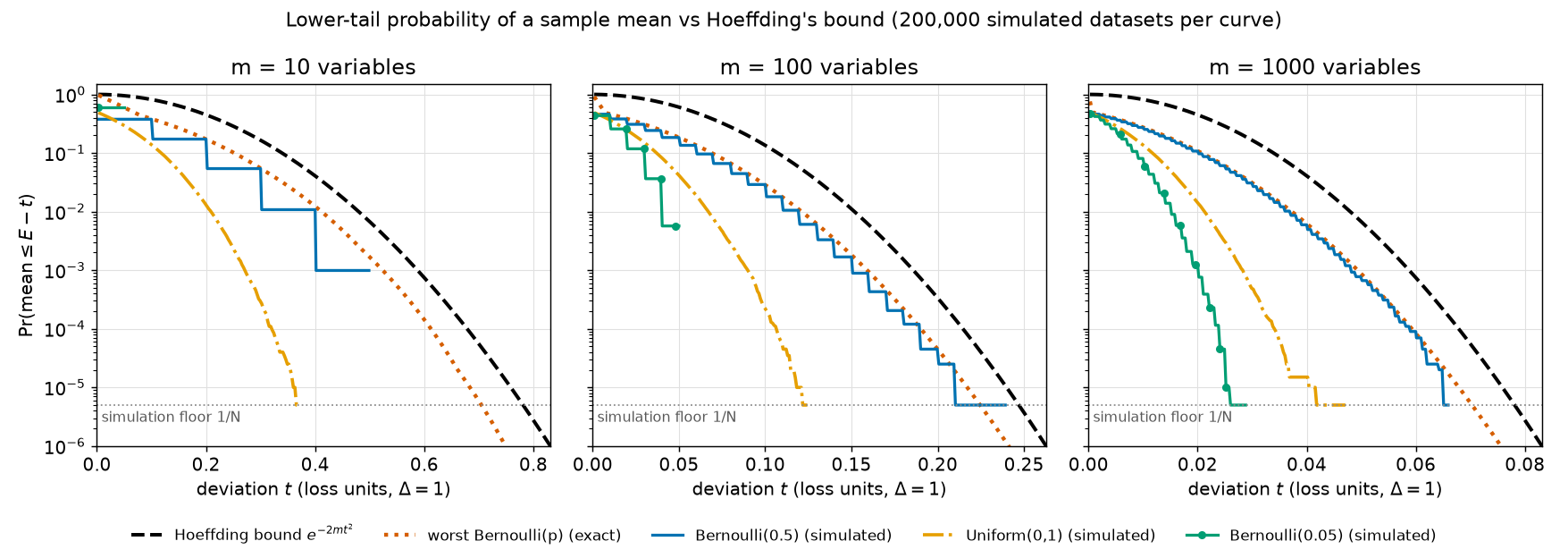
The figure plots, for \(m = 10\), 100 and 1000, the probability that the average falls \(t\) or more below its expected value, against the margin \(t\). The vertical axis is logarithmic, so each grid line is a factor of 10. A few rows of the underlying table (section [3] of the output):
| \(m\) | \(t\) | Hoeffding limit | Bernoulli(0.5) | Uniform(0,1) | Bernoulli(0.05) | worst Bernoulli |
|---|---|---|---|---|---|---|
| 10 | 0.30 | 1.65e-01 | 5.42e-02 | 2.90e-04 | 0 | 5.48e-02 |
| 100 | 0.10 | 1.35e-01 | 2.90e-02 | 2.20e-04 | 0 | 2.86e-02 |
| 1000 | 0.04 | 4.08e-02 | 5.96e-03 | 1.50e-05 | 0 | 6.23e-03 |
What to notice:
- Every curve stays under the dashed line. The script asserts this at 2730 grid points, allowing for the small random error of any simulation (Monte-Carlo noise).
- The worst case comes closest. Among all Bernoulli(\(p\)), the exact worst case (dotted) hugs the fair coin. Coins with outcomes only at the two ends of the interval are the hardest case for Hoeffding.
- Low-variance losses sit far below. Uniform(0,1) and Bernoulli(0.05) losses vary less than a fair coin, but Hoeffding's limit uses only the width \(\Delta\), not the spread. It cannot tell them apart.
- The steps in the coin curves appear because an average of \(m\) coins can only take the values \(0, 1/m, 2/m, \dots\).
The same looseness, measured as a margin (section [4]): at \(m = 1000\) Hoeffding asks for \(t = 0.0387\), while the margin that would actually have sufficed in the simulation was 0.0260 for the fair coin, 0.0150 for uniform losses and 0.0110 for Bernoulli(0.05).
Margins shrink like \(1/\sqrt m\): Hoeffding's \(t\) is 0.3870, 0.1224 and 0.0387 for \(m = 10\), 100 and 1000. Each tenfold increase in data shrinks the margin by a factor \(\sqrt{10}\), not 10.
Going deeper¶
Everything in this section is MY EXPLANATION unless tagged.
The proof takes three moves.
- Exponentiate, then use Markov's inequality. This needs the moment generating function.
- Limit each variable's moment generating function (Hoeffding's lemma), using the shape of the exponential curve.
- Multiply over the independent variables, then choose the best exponent.
Five terms carry the proof. Here they are in plain words; the collapsible blocks below prove everything.
The moment generating function (MGF) of a random variable \(Y\) is the function \(\lambda \mapsto \mathbb E[e^{\lambda Y}]\): for each real number \(\lambda\), the average value of \(e^{\lambda Y}\). It is called "moment generating" because its derivatives at \(\lambda = 0\) give \(\mathbb E[Y]\), \(\mathbb E[Y^2]\), and so on — the "moments" of \(Y\).
The Chernoff method bounds a tail probability \(\Pr(Y \ge c)\) in three steps. Pick a number \(\lambda > 0\). Note that \(Y \ge c\) happens exactly when \(e^{\lambda Y} \ge e^{\lambda c}\). Apply Markov's inequality to the positive quantity \(e^{\lambda Y}\) to get \(\Pr(Y \ge c) \le e^{-\lambda c}\,\mathbb E[e^{\lambda Y}]\). Finally choose the \(\lambda\) that makes the right side smallest.
A convex function is one whose graph, between any two of its points, lies on or below the straight segment (the chord) joining them. Bowl-shaped curves such as \(e^x\) and \(x^2\) are convex.
Jensen's inequality says that for a convex function \(f\) and a random variable \(Y\), \(f(\mathbb E Y) \le \mathbb E f(Y)\). In words: averaging first and then applying \(f\) gives a smaller number than applying \(f\) first and then averaging.
Hoeffding's lemma says: if a random variable \(Z\) always lies in \([a,b]\) and has expected value 0, then its MGF obeys \(\mathbb E[e^{\lambda Z}] \le \exp(\lambda^2(b-a)^2/8)\) for every real \(\lambda\). It is the heart of the proof.
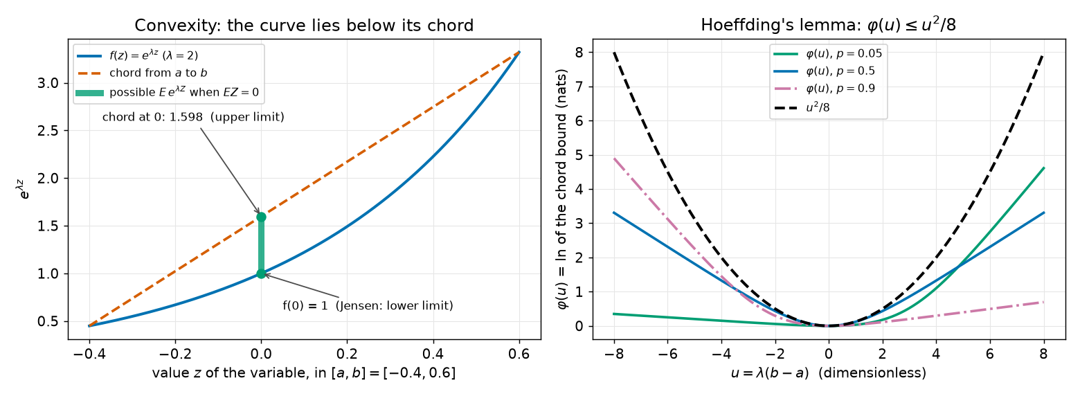
The left panel shows the two facts about convex curves that the proof uses. Jensen's inequality gives the lower end of the green bar; the chord gives the upper end. The right panel shows the function \(\varphi\) from the proof of Hoeffding's lemma staying under the parabola \(u^2/8\).
Going deeper: tools from Chapter 1, restated with proofs
These small facts are used repeatedly below.
(T1) Markov's inequality. If \(Y \ge 0\) always and \(c > 0\), then \(\Pr(Y \ge c) \le \mathbb E[Y]/c\). Proof: for every outcome, \(Y \ge c\,\mathbf 1[Y \ge c]\). (If \(Y \ge c\) the right side is \(c \le Y\); otherwise it is \(0 \le Y\).) Take expectations of both sides (using T2): \(\mathbb E Y \ge c\,\Pr(Y \ge c)\). Divide by \(c\).
(T2) Monotonicity of expectation. If \(Y \le W\) for every outcome, then \(\mathbb E Y \le \mathbb E W\). Proof: by linearity, \(\mathbb E W - \mathbb E Y = \mathbb E[W - Y]\), and the expectation of a quantity that is never negative is a sum (or integral) of non-negative terms, hence non-negative.
(T3) Products of independent variables. If \(Z_1, \dots, Z_m\) are independent and \(g_1, \dots, g_m\) are functions, then
Proof by induction on \(m\). For \(m = 1\) there is nothing to prove. Suppose it holds for \(k\) factors. The product of the first \(k\) factors is a function of \((Z_1, \dots, Z_k)\) alone, so it is independent of \(g_{k+1}(Z_{k+1})\). Chapter 1's product rule for two independent variables gives \(\mathbb E[\prod_{i\le k+1}] = \mathbb E[\prod_{i \le k}]\cdot \mathbb E[g_{k+1}(Z_{k+1})]\), and the induction hypothesis finishes the step.
(T4) Continuous variables. For a variable with a density (such as Uniform(0,1)), expectations are integrals instead of sums. T1–T3 hold with the same proofs.
(T5) Complements. \(\Pr(\text{not } A) = 1 - \Pr(A)\), from additivity of probability over the disjoint events \(A\) and "not \(A\)".
Going deeper: the moment generating function and the Chernoff method
Definition. The MGF of a random variable \(Y\) is \(M_Y(\lambda) = \mathbb E[e^{\lambda Y}]\) for real \(\lambda\). If \(Y\) is bounded, \(e^{\lambda Y}\) is bounded too, so \(M_Y(\lambda)\) is finite for every \(\lambda\). The units of \(\lambda\) are "one over the units of \(Y\)", so that \(\lambda Y\) is a pure number.
Why "moment generating". Expand the exponential as a power series, \(e^{\lambda Y} = \sum_{k\ge0} (\lambda Y)^k/k!\). For bounded \(Y\) the expectation can be taken term by term:
so the \(k\)-th derivative of \(M_Y\) at \(\lambda = 0\) is \(\mathbb E[Y^k]\), the \(k\)-th moment.
Two properties we need.
- Shift: \(M_{Y-c}(\lambda) = \mathbb E[e^{\lambda Y}e^{-\lambda c}] = e^{-\lambda c}M_Y(\lambda)\) (linearity).
- Independent sums: if \(Y_1, \dots, Y_m\) are independent, then \(M_{Y_1+\dots+Y_m}(\lambda) = \mathbb E[\prod_i e^{\lambda Y_i}] = \prod_i M_{Y_i}(\lambda)\), by T3 with \(g_i(y) = e^{\lambda y}\).
Example: a Bernoulli(\(p\)) variable has \(M(\lambda) = (1-p)e^{0} + p e^{\lambda} = 1 - p + p e^{\lambda}\). This expression reappears in Hoeffding's lemma.
The Chernoff bound. For any real \(c\) and any \(\lambda > 0\),
Proof. The map \(y \mapsto e^{\lambda y}\) is strictly increasing when \(\lambda > 0\), so the events \(\{Y \ge c\}\) and \(\{e^{\lambda Y} \ge e^{\lambda c}\}\) are the same event. The variable \(e^{\lambda Y}\) is positive and \(e^{\lambda c} > 0\), so Markov's inequality (T1) gives \(\Pr(e^{\lambda Y} \ge e^{\lambda c}) \le \mathbb E[e^{\lambda Y}]/e^{\lambda c}\). Since this holds for every \(\lambda > 0\), we may use the \(\lambda\) that makes the right side smallest. These are the three steps of the Chernoff method: exponentiate, apply Markov, optimize \(\lambda\).
Why it beats Chebyshev. Chebyshev's inequality is Markov applied to \((Y - \mathbb E Y)^2\); it uses only the second moment. The Chernoff method applies Markov to \(e^{\lambda Y}\), which contains all moments at once. For a sum of independent variables the MGF factorizes into a product, and a product of \(m\) factors each a little above 1 is what produces a limit that falls exponentially in \(m\).
Why \(\lambda > 0\). For \(\lambda < 0\) the map \(y \mapsto e^{\lambda y}\) is decreasing, so the event flips to \(\{Y \le c\}\). The lower tail can be handled that way, or (as below) by applying the upper-tail result to \(-Y\).
Going deeper: convex functions and Jensen's inequality, with proofs
Definition. A function \(f\) on an interval \(I\) is convex if for all \(x, y \in I\) and all \(\gamma \in [0,1]\),
As \(\gamma\) runs from 0 to 1, the point \(\gamma x + (1-\gamma)y\) runs along the segment from \(y\) to \(x\), and the right side runs along the chord between \((y, f(y))\) and \((x, f(x))\). So the definition says: the graph lies on or below every chord.
Fact C1 (second-derivative test). If \(f\) is twice differentiable on \(I\) and \(f'' \ge 0\) there, then \(f\) is convex. Proof. Take \(x < y\) in \(I\), \(\gamma \in (0,1)\) (the cases \(\gamma = 0, 1\) hold with equality), and \(z = \gamma x + (1-\gamma)y\), so \(x < z < y\), \(z - x = (1-\gamma)(y-x)\) and \(y - z = \gamma(y-x)\). By the mean value theorem there are \(\xi_1 \in (x,z)\) and \(\xi_2 \in (z,y)\) with \(f(z) - f(x) = f'(\xi_1)(z-x)\) and \(f(y) - f(z) = f'(\xi_2)(y-z)\). Because \(f'' \ge 0\), \(f'\) is non-decreasing, and \(\xi_1 < \xi_2\) gives \(f'(\xi_1) \le f'(\xi_2)\). Hence
Multiply by \(\gamma(1-\gamma) > 0\): \(\gamma f(z) - \gamma f(x) \le (1-\gamma) f(y) - (1-\gamma) f(z)\). Collect the \(f(z)\) terms: \(f(z) \le \gamma f(x) + (1-\gamma) f(y)\). \(\square\)
Consequences: \(e^{\lambda z}\) is convex in \(z\) for every real \(\lambda\) (second derivative \(\lambda^2 e^{\lambda z} \ge 0\)); \(z^2\) is convex (second derivative 2); \(-\ln z\) is convex on \((0,\infty)\) (second derivative \(1/z^2\)).
Fact C2 (the tangent line lies below the graph). If \(f\) is convex on \(I\) and differentiable at an interior point \(\mu\), then \(f(z) \ge f(\mu) + f'(\mu)(z - \mu)\) for every \(z \in I\). Proof. Fix \(z \ne \mu\) and \(\gamma \in (0,1]\). Convexity with the points \(z\) and \(\mu\) gives \(f(\mu + \gamma(z-\mu)) = f(\gamma z + (1-\gamma)\mu) \le \gamma f(z) + (1-\gamma) f(\mu)\). Subtract \(f(\mu)\) and divide by \(\gamma > 0\):
As \(\gamma \to 0^+\), the left side tends to \(f'(\mu)(z - \mu)\) (definition of the derivative). The inequality survives the limit, so \(f'(\mu)(z-\mu) \le f(z) - f(\mu)\). \(\square\)
Jensen's inequality. Let \(f\) be convex and differentiable on an open interval \(I\), and let \(Y\) take values in \(I\) with finite expected value \(\mu = \mathbb E Y\) (then \(\mu \in I\)). Then
Proof. Apply C2 at \(\mu\) with \(z = Y\); it holds for every outcome: \(f(Y) \ge f(\mu) + f'(\mu)(Y - \mu)\). Take expectations, using monotonicity (T2) and linearity: \(\mathbb E f(Y) \ge f(\mu) + f'(\mu)(\mathbb E Y - \mu) = f(\mu)\). \(\square\) The line \(f(\mu) + f'(\mu)(z-\mu)\) is called a supporting line: it touches the graph at \(\mu\) and stays below it. For a convex function without a derivative at \(\mu\), any slope between the left and right derivatives (which always exist for convex functions) gives a supporting line, and the same proof works. Every function in this explainer is differentiable, so we skip that case.
Two examples. With \(f(y) = y^2\): \((\mathbb E Y)^2 \le \mathbb E Y^2\), which says variance is never negative. With \(f(y) = e^{\lambda y}\) and \(\mathbb E Y = 0\): \(\mathbb E e^{\lambda Y} \ge e^0 = 1\), the lower end of the green bar in the figure. Chapter 17 uses Jensen again to compare sampling with and without replacement.
The chord bound (the other side). Now suppose \(Y\) always lies in a closed interval \([a,b]\) with \(a < b\), and \(f\) is convex on \([a,b]\). Each \(y \in [a,b]\) can be written as \(y = \gamma a + (1-\gamma)b\) with \(\gamma = (b-y)/(b-a) \in [0,1]\). Convexity gives, for every outcome,
The right side is a straight-line function of \(Y\), so taking expectations (T2, linearity) replaces \(Y\) by \(\mathbb E Y\):
Together with Jensen, \(\mathbb E f(Y)\) is sandwiched between \(f(\mathbb E Y)\) and the chord's height at \(\mathbb E Y\). Jensen holds for any variable; the chord bound needs the variable to be confined to \([a,b]\). That confinement is where Hoeffding's boundedness requirement enters.
Going deeper: proof of Hoeffding's lemma
Statement. Let \(Z\) be a random variable with \(a \le Z \le b\) always and \(\mathbb E Z = 0\). Then for every real \(\lambda\),
Units: \(\lambda\) is in "one over the units of \(Z\)", so \(\lambda Z\) and \(\lambda(b-a)\) are pure numbers.
Step 0: the interval contains 0. Since \(Z \ge a\) always, \(0 = \mathbb E Z \ge a\) (T2). Likewise \(b \ge 0\). If \(a = b\), then \(a = b = 0\), so \(Z = 0\) always and both sides equal 1. From now on \(a < b\).
Step 1: the chord. The function \(z \mapsto e^{\lambda z}\) is convex (Fact C1). By the chord bound with \(\mathbb E Z = 0\):
Step 2: rename. Let \(p = -a/(b-a)\). Then \(1 - p = b/(b-a)\), and both lie in \([0,1]\) because \(a \le 0 \le b\). (Interpretation: \(p\) is the probability that a variable taking only the values \(a\) and \(b\) must put on \(b\) to have mean 0.) Let \(u = \lambda(b-a)\). Because \(a = -p(b-a)\), we get \(\lambda a = -pu\), and \(\lambda b = \lambda a + \lambda(b-a) = (1-p)u\). The right side of Step 1 becomes
The bracket is positive, so we can take its logarithm and write the right side as \(e^{\varphi(u)}\) with
Step 3: value and slope at 0. \(\varphi(0) = 0 + \ln 1 = 0\). Differentiating,
At \(u = 0\), \(q(0) = p\), so \(\varphi'(0) = 0\).
Step 4: curvature at most 1/4. By the quotient rule,
using \(1 - q(u) = (1-p)/(1 - p + p e^{u})\). Completing the square, \(q(1-q) = \tfrac14 - (q - \tfrac12)^2 \le \tfrac14\). So \(\varphi''(u) \le 1/4\) for every \(u\).
Step 5: Taylor. Taylor's theorem with the Lagrange remainder says there is a \(\xi\) between 0 and \(u\) with
The same conclusion without Taylor's theorem: let \(g(u) = u^2/8 - \varphi(u)\). Then \(g(0) = 0\), \(g'(0) = 0\) and \(g''(u) = 1/4 - \varphi''(u) \ge 0\). So \(g'\) is non-decreasing: \(g'(u) \ge g'(0) = 0\) for \(u \ge 0\) and \(g'(u) \le 0\) for \(u \le 0\). So \(g\) is non-increasing on \((-\infty, 0]\) and non-decreasing on \([0, \infty)\); its smallest value is \(g(0) = 0\). Hence \(\varphi(u) \le u^2/8\).
Step 6: conclude. \(\mathbb E[e^{\lambda Z}] \le e^{\varphi(u)} \le e^{u^2/8} = \exp(\lambda^2(b-a)^2/8)\). \(\square\)
Numerical check (output section [5]). On a grid of \(p \in [0.001, 0.999]\) and \(u \in [-30, 30]\) the largest value of \(\varphi(u) - u^2/8\) is 0, reached at \(u = 0\), and the largest \(\varphi''\) is 0.2500. For three mean-zero variables in an interval of width 1 the script compares the MGF with the lemma's limit:
| \(\lambda\) | two-point, \(p = 0.5\) | uniform | two-point, \(p = 0.05\) | limit \(e^{\lambda^2/8}\) |
|---|---|---|---|---|
| 0.5 | 1.0314 | 1.0104 | 1.0069 | 1.0317 |
| 2.0 | 1.5431 | 1.1752 | 1.1939 | 1.6487 |
| 8.0 | 27.3082 | 6.8225 | 100.5466 | 2980.9580 |
What the 1/8 means. For small \(\lambda\) the expansion of the MGF with \(\mathbb E Z = 0\) gives \(\mathbb E e^{\lambda Z} \approx 1 + \lambda^2\mathrm{Var}(Z)/2\), while the limit is \(e^{\lambda^2(b-a)^2/8} \approx 1 + (\lambda^2/2)\cdot(b-a)^2/4\). So the lemma treats \(Z\) as if its variance were \((b-a)^2/4\) — the largest variance any variable confined to \([a,b]\) can have (shown for width 1 in the first deeper block; rescale for other widths). A fair two-point variable has exactly that variance, which is why its column nearly equals the limit at \(\lambda = 0.5\). Lower-variance variables sit well below it.
Going deeper: proof of Hoeffding's inequality (all versions)
Statement (upper tail). Let \(Z_1, \dots, Z_m\) be independent with \(a_i \le Z_i \le b_i\) always, let \(S = \sum_i Z_i\), and let \(W = \sum_i (b_i - a_i)^2 > 0\). Then for every \(\varepsilon > 0\), \(\Pr(S - \mathbb E S \ge \varepsilon) \le \exp(-2\varepsilon^2/W)\).
(a) Centre. Let \(Y_i = Z_i - \mathbb E Z_i\). Then \(\mathbb E Y_i = 0\), and \(Y_i\) lies in \([a_i - \mathbb E Z_i,\ b_i - \mathbb E Z_i]\), an interval of the same width \(w_i = b_i - a_i\). By linearity, \(S - \mathbb E S = \sum_i Y_i\). The \(Y_i\) are independent, being functions of independent variables.
(b) Chernoff. Fix \(\lambda > 0\). By the Chernoff bound,
(c) Factorize. \(e^{\lambda \sum_i Y_i} = \prod_i e^{\lambda Y_i}\), and by independence (T3) \(\mathbb E[\prod_i e^{\lambda Y_i}] = \prod_i \mathbb E[e^{\lambda Y_i}]\). This is the only place independence is used.
(d) Hoeffding's lemma for each \(Y_i\) (mean 0, width \(w_i\)): \(\mathbb E[e^{\lambda Y_i}] \le e^{\lambda^2 w_i^2/8}\). All factors are positive, so the product of the limits limits the product:
(e) Optimize \(\lambda\). The exponent \(h(\lambda) = -\lambda\varepsilon + \lambda^2 W/8\) is a parabola opening upwards. Its derivative \(h'(\lambda) = -\varepsilon + \lambda W/4\) vanishes at \(\lambda^* = 4\varepsilon/W\), which is positive, so it is allowed. The value there is
Hence \(\Pr(S - \mathbb E S \ge \varepsilon) \le e^{-2\varepsilon^2/W}\). \(\square\)
Lower tail. Apply the upper tail to \(Z_i' = -Z_i\), which lies in \([-b_i, -a_i]\), an interval of the same width. With \(S' = -S\), the event \(\{S - \mathbb E S \le -\varepsilon\}\) is the event \(\{S' - \mathbb E S' \ge \varepsilon\}\), so it has the same limit \(e^{-2\varepsilon^2/W}\).
Two-sided. For \(\varepsilon > 0\) the events \(A = \{S - \mathbb E S \ge \varepsilon\}\) and \(B = \{S - \mathbb E S \le -\varepsilon\}\) cannot both happen. By additivity for disjoint events (Chapter 1), \(\Pr(\lvert S - \mathbb E S\rvert \ge \varepsilon) = \Pr(A) + \Pr(B) \le 2e^{-2\varepsilon^2/W}\). No union bound is needed here.
Mean form. If every width is \(\Delta\), then \(W = m\Delta^2\). With \(\bar Z = S/m\), the event \(\{\bar Z \le \mathbb E\bar Z - t\}\) is the event \(\{S - \mathbb E S \le -mt\}\). Put \(\varepsilon = mt\):
Confidence form. Let \(t_\delta = \Delta\sqrt{\ln(1/\delta)/(2m)}\). Then \(2mt_\delta^2/\Delta^2 = \ln(1/\delta)\), so the limit equals \(e^{-\ln(1/\delta)} = \delta\). By T5, \(\Pr(\bar Z > \mathbb E\bar Z - t_\delta) \ge 1 - \delta\), which rearranges to \(\Pr(\mathbb E\bar Z < \bar Z + t_\delta) \ge 1 - \delta\).
Units, tracked. \(\varepsilon\) and \(w_i\) are in loss units, \(W\) in loss units squared, so \(\varepsilon^2/W\) is a pure number. \(\lambda\) is in one over loss units. In the mean form the best \(\lambda\) is \(\lambda^* = 4mt/(m\Delta^2) = 4t/\Delta^2\). In worked example (a) this is 0.4895 per loss unit. That is a small value, where the lemma is nearly exact for a fair coin (the \(\lambda = 0.5\) row above: 1.0314 against 1.0317).
Going deeper: how tight is Hoeffding's inequality?
Fair coins: the exponent is almost exactly right. Write \(\mathrm{kl}(x\,\Vert\,y) = x\ln\frac{x}{y} + (1-x)\ln\frac{1-x}{1-y}\) (in nats) for how different a coin of bias \(x\) is from one of bias \(y\). SOURCE: Hoeffding 1963, Theorem 1 For variables in \([0,1]\) with mean \(\mu\), Hoeffding's original paper first proves the sharper limit \(\exp(-m\,\mathrm{kl}(\mu - t\,\Vert\,\mu))\) for the lower tail and only then loosens it to \(e^{-2mt^2}\). MY EXPLANATION We do not derive it here; the script only evaluates it (output section [6]):
| case | sharper exponent \(m\,\mathrm{kl}\) | Hoeffding exponent \(2mt^2\) | exact tail |
|---|---|---|---|
| Bernoulli(0.5), \(m = 100\), \(t = 0.1\) | 2.0136 | 2.0000 | 2.84e-02 |
| Bernoulli(0.05), \(m = 100\), \(t = 0.04\) | 2.4736 | 0.3200 | 3.71e-02 |
For the fair coin the two exponents nearly agree. The remaining gap between the exact tail (2.84e-02) and \(e^{-2} = 0.1353\) is lost in the Markov step: Markov's inequality is wasteful by a factor that does not grow exponentially with \(m\).
Low-variance losses: Hoeffding is loose. For Bernoulli(0.05) the sharper exponent (2.4736) is many times Hoeffding's (0.3200). The reason is the lemma's worst-case variance \((b-a)^2/4\): a Bernoulli(0.05) loss has a much smaller variance, but Hoeffding only sees the width. In margin terms (output section [4]), at \(m = 1000\) Hoeffding asks for 0.0387 where 0.0110 sufficed.
Variance-aware alternatives (named, not derived). Bernstein's inequality uses both the range and the variance. The kl form above is sharper for losses near 0 or 1. SOURCE: Lotfi et al. 2022, §3 and App. J.1 The earlier compression-bound paper by the same group used Catoni's PAC-Bayes bound, which is tighter when the training error is small. PAPER §A.1, p. 12 This paper uses plain Hoeffding.
MY EXPLANATION Why this matters for the paper. For bits per token the width is the worst case, \(\Delta = 18.787\) bits/token at \(\alpha = 0.1\), while each document's loss is an average over many tokens. If document losses in practice spread over a much narrower range than \(\Delta\), Hoeffding still charges for the full width. A variance-sensitive bound could shrink the margin; the paper does not explore this.
Going deeper: edge cases and fine print
- \(\varepsilon\) must be positive. At \(\varepsilon = 0\) the limit is 1, which says nothing. For \(\varepsilon < 0\) the formula would give a number below 1 for an event that can have probability 1 (for example when every \(Z_i\) is constant), so the theorem makes no claim there. The paper's "for any \(t > 0\)" respects this.
- Zero total width. If \(W = 0\), every \(Z_i\) is constant and \(\Pr(S - \mathbb E S \ge \varepsilon) = 0\). Step (d) then gives \(e^{-\lambda\varepsilon}\) for every \(\lambda > 0\), which tends to 0 as \(\lambda \to \infty\); read the formula as \(e^{-\infty} = 0\).
- "\(\ge\)" versus "\(>\)". The limit for \(\{S - \mathbb E S \ge \varepsilon\}\) also covers the smaller event \(\{S - \mathbb E S > \varepsilon\}\). The paper's event \(R(h) \ge \hat R(h) + t\) is the non-strict version, which matches.
- The interval must hold always and be fixed in advance. An interval read off the data (say, the smallest and largest observed loss) is not allowed: it is random, and a future value may fall outside it.
- Different distributions and widths are fine. The general form only needs \(\sum_i (b_i - a_i)^2\).
- Conditional use (App. A.3; Chapter 17). If, given some information \(G\) (for example, the training set), the variables are independent and bounded, the inequality holds conditionally on each value of \(G\), with conditional expectations in place of expectations. Averaging the conditional probability over \(G\) (the tower rule of Chapter 1) gives the same limit without conditioning.
- Sampling without replacement. Draws without replacement are dependent, so step (c) fails as written. Hoeffding (1963, Theorem 4) shows that the same limit still holds; Chapter 17 proves it (erratum E05).
- Data-dependent hypothesis. If \(\hat h\) is chosen using \(X_1, \dots, X_m\), then \(Z_j = R(\hat h, X_j)\) depends on all the documents, so step (c) fails, and in general \(\mathbb E[\hat R(\hat h)] \ne R(\hat h)\). Chapter 10 repairs this.
Common misconceptions¶
Everything in this section is MY EXPLANATION.
- Misconception: Hoeffding's inequality requires i.i.d. data. — Actually: it requires only independence and boundedness; each variable may have its own distribution and its own interval. The paper needs "identically distributed" for a different reason: so that the expected value of \(\hat R(h)\) is the population risk \(R(h)\) (Chapter 15).
- Misconception: "With probability 95 %, the true loss is below training loss plus \(t\)" is a statement about my particular training set. — Actually: the probability is over the random draw of the training set. For the set you actually have, the statement is either true or false; 95 % is the success rate of the procedure.
- Misconception: The guarantee applies to the model I just trained. — Actually: it applies only to a hypothesis fixed before the data were seen. A trained model was chosen using the data, which breaks independence; Chapter 10 pays for that choice.
- Misconception: Hoeffding's limit is close to the true probability. — Actually: it is a worst case over every distribution in the interval and ignores the variance. For Bernoulli(0.05) losses at \(m = 1000\) it asks for a margin of 0.0387 where 0.0110 sufficed.
- Misconception: Doubling the data halves the margin. — Actually: the margin shrinks like \(1/\sqrt m\): 0.3870, 0.1224 and 0.0387 for \(m = 10\), 100 and 1000. Halving the margin needs four times the data.
- Misconception: Only the size of \(t\) matters. — Actually: only \(t/\Delta\) matters. A loss with a wide range needs a proportionally wider margin: 0.0081 bits/token for \(\Delta = 18.787\) bits/token versus 0.000432 for \(\Delta = 1\), at the same \(m\) and \(\delta\). That is why the smoothing weight \(\alpha\), which sets \(\Delta\), matters (Chapter 16).
Self-test¶
Q1. With prediction smoothing at \(\alpha = 0.1\) the per-document loss lies in an interval of width \(\Delta = 18.787\) bits/token. For one hypothesis fixed in advance, how many independent documents does Hoeffding need to guarantee, with \(\delta = 0.05\), that the expected loss is at most the empirical risk plus \(t = 0.01\) bits/token?
Answer
We need \(\Delta\sqrt{\ln(1/\delta)/(2m)} \le t\). Square both sides and solve for \(m\):
With \(\Delta = 18.787\) bits/token, \(\ln(1/0.05) = 2.995732\) nats and \(t = 0.01\) bits/token, the bits/token units
cancel and the script gives \(m \ge 5{,}286{,}719.4\), so 5,286,720 documents. OpenWebText has more, 8,009,762
[SOURCE: nanoGPT prepare.py split], which is why worked example (b) found a margin of 0.0081, below 0.01.
Q2. Someone writes: "with probability at least 0.95, \(R(h) \le \hat R(h) + 0.0081\) bits/token". What is random, what is fixed, and why can this sentence fail for a model that was trained on the same documents?
Answer
Random: the \(m\) training documents, and therefore the empirical risk \(\hat R(h)\). Fixed: the hypothesis \(h\), its expected risk \(R(h)\), the margin 0.0081, the width \(\Delta\), \(m\) and \(\delta\). The "0.95" is the fraction of repeated draws of the training set in which the sentence comes out true. For a trained model, \(h\) was chosen by looking at the documents — typically because it has a low loss on them. The losses \(R(h, X_j)\) then all depend on every document, so they are not independent, and \(\mathbb E[\hat R(h)]\) need not equal \(R(h)\). Hoeffding's requirement "fixed in advance" fails. Chapter 10 repairs this with a union bound over all hypotheses that could have been chosen.
Q3. Let \(Z_1 = Z_2 = \dots = Z_{100}\) all be the same fair coin (0 or 1). Which requirement of Hoeffding's inequality fails? Compare the true value of \(\Pr(\bar Z \le 0.2)\) with what the formula would claim at \(t = 0.3\), and say which step of the proof breaks.
Answer
Independence fails: knowing \(Z_1\) tells you every other \(Z_i\). The average equals \(Z_1\), so \(\Pr(\bar Z \le 0.2) = \Pr(Z_1 = 0) = 0.5\). The formula would claim at most \(\exp(-2 \cdot 100 \cdot 0.3^2) = e^{-18} = 1.52\times 10^{-8}\), which is wildly false. The broken step is (c), the factorization: \(\mathbb E[e^{\lambda S}] = \mathbb E[e^{100\lambda Z_1}]\), which is not the product of 100 separate factors \(\mathbb E[e^{\lambda Z_i}]\). Without independence there is no cancellation — the crowd pushes as one.
Code for this chapter¶
Run it from the project root:
.venv/Scripts/python explainer/code/ch09_hoeffding.py
Source: ch09_hoeffding.py
"""Chapter 9 demo: Hoeffding's inequality, checked by simulation.

Claims reproduced / illustrated
  * Hoeffding's inequality, lower tail, for the mean of m independent variables in [0, 1]
    (interval width Delta = 1):   P(mean <= E - t) <= exp(-2 m t^2).
    This is the step used in the proof of Theorem A.1 (paper App. A.1, p. 12) and again in
    App. A.3 (p. 14).  Checked by simulating 200,000 datasets for Bernoulli(0.5),
    Uniform(0,1), Bernoulli(0.05), plus the exact worst case over all Bernoulli(p).
  * Inversion: with probability >= 1 - delta (over the draw of the m samples),
    E <= mean + Delta * sqrt(ln(1/delta) / (2m)).  Coverage is checked by simulation.
  * Why an exponential tail matters: Hoeffding vs Chebyshev at tiny failure probabilities.
  * Hoeffding's lemma numerically: phi(u) <= u^2/8 and phi'' <= 1/4.
  * Worked-example numbers of Chapter 9: m = 100; and the paper's scale
    m = 8,009,762 [SOURCE nanoGPT / authors' code], delta = 0.05 [SOURCE authors' code],
    Delta = 18.787 bits/token for alpha = 0.1 (Theorem A.2, via pacbound.smoothing_interval).

Outputs: code/outputs/ch09_hoeffding.txt,
         docs/assets/fig/ch09_hoeffding_tails.png, docs/assets/fig/ch09_convexity.png
"""
from __future__ import annotations

import math
import sys
import time
from pathlib import Path

import numpy as np
from scipy.stats import binom

import matplotlib
matplotlib.use("Agg")
import matplotlib.pyplot as plt

HERE = Path(__file__).resolve().parent
sys.path.insert(0, str(HERE))
import pacbound as pb  # noqa: E402

OUT_TXT = HERE / "outputs" / "ch09_hoeffding.txt"
FIG_DIR = HERE.parent / "docs" / "assets" / "fig"
FIG_TAILS = FIG_DIR / "ch09_hoeffding_tails.png"
FIG_CONVEX = FIG_DIR / "ch09_convexity.png"

N_SIM = 200_000            # simulated datasets per (distribution, m)
MS = [10, 100, 1000]       # number of variables per dataset
DELTA = pb.DELTA           # 0.05 [SOURCE authors' code]
CHUNK = 10_000             # datasets per chunk for the Uniform simulation (memory)

lines: list[str] = []


def out(s: str = "") -> None:
    print(s)
    lines.append(s)


def fmt_p(x: float) -> str:
    """Probability in compact scientific notation; exact zero printed as 0."""
    return "0" if x == 0 else f"{x:.2e}"


# ---------------------------------------------------------------------------
# Simulation of sample means (all variables take values in [0, 1])
# ---------------------------------------------------------------------------
def simulate_means(rng: np.random.Generator, dist: str, m: int) -> np.ndarray:
    """Return N_SIM sample means of m independent draws; sorted ascending."""
    if dist == "bern0.5":
        means = rng.binomial(m, 0.5, size=N_SIM) / m
    elif dist == "bern0.05":
        means = rng.binomial(m, 0.05, size=N_SIM) / m
    elif dist == "unif":
        parts = [rng.random((CHUNK, m)).mean(axis=1) for _ in range(N_SIM // CHUNK)]
        means = np.concatenate(parts)
    else:
        raise ValueError(dist)
    return np.sort(means)


def tail_le(sorted_means: np.ndarray, x: np.ndarray) -> np.ndarray:
    """Empirical P(mean <= x) (tiny tolerance so exact ties count as <=)."""
    return np.searchsorted(sorted_means, x + 1e-12, side="right") / sorted_means.size


def tail_lt(sorted_means: np.ndarray, x: float) -> float:
    """Empirical P(mean < x)."""
    return np.searchsorted(sorted_means, x, side="left") / sorted_means.size


def worst_bernoulli_tail(m: int, t: float) -> float:
    """Exact sup over p in [0,1] of P(K/m <= p - t), K ~ Binomial(m, p).
    For p in [t + k/m, t + (k+1)/m) the event is {K <= k}, whose probability falls as
    p grows, so the sup is max_k P(K <= k) at p = t + k/m (needs p <= 1).
    The same value is the sup of the strict version P(K/m < p - t)."""
    k = np.arange(0, m + 1)
    p = t + k / m
    ok = p <= 1.0
    if not ok.any():
        return 0.0
    return float(binom.cdf(k[ok], m, p[ok]).max())


def kl_bern(a: float, b: float) -> float:
    """Binary relative entropy kl(a || b) in nats (0 < b < 1, 0 <= a <= 1)."""
    s = 0.0
    if a > 0:
        s += a * math.log(a / b)
    if a < 1:
        s += (1 - a) * math.log((1 - a) / (1 - b))
    return s


DISTS = [("bern0.5", "Bernoulli(0.5)", 0.5),
         ("unif", "Uniform(0,1)", 0.5),
         ("bern0.05", "Bernoulli(0.05)", 0.05)]


def main() -> None:
    t0 = time.time()
    rng = np.random.default_rng(0)
    FIG_DIR.mkdir(parents=True, exist_ok=True)
    OUT_TXT.parent.mkdir(parents=True, exist_ok=True)

    out("Chapter 9 - Hoeffding's inequality: worked numbers and simulation")
    out("=" * 66)

    # ---------------- [1] worked examples ----------------
    out("[1] Worked examples (one FIXED hypothesis; t in loss units)")
    ln_inv_d = math.log(1.0 / DELTA)
    t_a = pb.hoeffding_t(100, 1.0, ln_inv_d)
    t_a2 = pb.hoeffding_t(100, 1.0, math.log(2.0 / DELTA))
    out(f"  (a) m = 100, Delta = 1, delta = 0.05: ln(1/delta) = {ln_inv_d:.6f} nats")
    out(f"      one-sided t = sqrt(ln 20 / 200) = {t_a:.4f}   two-sided t = sqrt(ln 40 / 200) = {t_a2:.4f}")
    out(f"      bound at t = 0.1: exp(-2*100*0.1^2) = exp(-2) = {pb.hoeffding_tail(0.1, 100, 1.0):.4f}")
    out(f"      Chernoff's best lambda* = 4 t / Delta^2 = {4 * t_a:.4f} per loss unit (at t = {t_a:.4f})")
    m = pb.M_DOCS
    t_b1 = pb.hoeffding_t(m, 1.0, ln_inv_d)
    _, _, width = pb.smoothing_interval(0.1)
    t_b2 = pb.hoeffding_t(m, width, ln_inv_d)
    out(f"  (b) m = {m:,} documents [SOURCE nanoGPT split], delta = 0.05 [SOURCE authors' code]")
    out(f"      Delta = 1 (top-k error, fraction):        t = {t_b1:.6f}")
    out(f"      Delta = {width:.3f} bits/token (alpha = 0.1):  t = {t_b2:.4f} bits/token")
    # sum form used in the paper's proof: eps = m t, sum of squared widths = m Delta^2
    eps, ssq = m * t_b2, m * width ** 2
    same = math.exp(-2 * eps ** 2 / ssq)
    assert abs(same - DELTA) < 1e-9 and abs(pb.hoeffding_tail(t_b2, m, width) - DELTA) < 1e-9
    out(f"      sum form: exp(-2 (m t)^2 / (m Delta^2)) = {same:.6f} = delta  (check OK)")
    assert round(t_a, 4) == 0.1224 and round(t_b1, 6) == 0.000432 and round(t_b2, 4) == 0.0081

    # ---------------- [2] Hoeffding vs Chebyshev ----------------
    out("")
    out(f"[2] Deviation t needed for failure probability d' (m = {m:,}, losses in [0,1])")
    out("    Hoeffding: sqrt(ln(1/d')/(2m))   Chebyshev (Var <= 1/4): sqrt(1/(4 m d'))")
    for label, log10_d in [("0.05", math.log10(0.05)), ("1e-6", -6.0),
                           ("0.05 * 2^-1000", math.log10(0.05) - 1000 * math.log10(2.0))]:
        ln_inv = -log10_d * math.log(10.0)
        th = math.sqrt(ln_inv / (2 * m))
        log10_tc = 0.5 * (-math.log10(4 * m) - log10_d)
        tc = f"{10 ** log10_tc:.6f}" if log10_tc < 2 else f"10^{log10_tc:.1f}  (vacuous: > 1)"
        out(f"    d' = {label:<15} Hoeffding t = {th:.6f}   Chebyshev t = {tc}")

    # ---------------- [3] simulated tails ----------------
    out("")
    out(f"[3] Lower tail Pr(mean <= E - t): {N_SIM:,} simulated datasets per cell (seed 0)")
    out("    bound = exp(-2 m t^2);  'worst' = exact sup over all Bernoulli(p)")
    out(f"    {'m':>5} {'t':>5} {'bound':>9} {'Bern(0.5)':>10} {'Unif(0,1)':>10} {'Bern(0.05)':>10} {'worst':>9}")
    show_t = {10: [0.1, 0.2, 0.3, 0.4], 100: [0.05, 0.1, 0.15], 1000: [0.02, 0.04, 0.06]}
    grids, sims, worst_curves, bounds = {}, {}, {}, {}
    n_checked = 0
    for mm in MS:
        tmax = math.sqrt(math.log(1e6) / (2 * mm))
        tg = np.linspace(tmax / 300, tmax, 300)
        tg = np.unique(np.concatenate([tg, show_t[mm]]))
        bnd = np.exp(-2 * mm * tg ** 2)
        grids[mm], bounds[mm] = tg, bnd
        sims[mm] = {}
        for key, _, mean in DISTS:
            s = simulate_means(rng, key, mm)
            emp = tail_le(s, mean - tg)
            sims[mm][key] = (s, emp)
            # Monte-Carlo allowance: 4 standard errors at the bound + 2 counts
            allow = 4 * np.sqrt(bnd * (1 - bnd) / N_SIM) + 2.0 / N_SIM
            assert np.all(emp <= bnd + allow), (key, mm)
            n_checked += tg.size
            if key.startswith("bern"):   # simulation agrees with exact binomial
                p = 0.5 if key == "bern0.5" else 0.05
                exact = binom.cdf(np.floor(mm * (p - tg) + 1e-9), mm, p)
                se = np.sqrt(exact * (1 - exact) / N_SIM) + 1.0 / N_SIM
                assert np.all(np.abs(emp - exact) <= 5 * se), (key, mm)
        worst = np.array([worst_bernoulli_tail(mm, t) for t in tg])
        assert np.all(worst <= bnd + 1e-12), mm
        worst_curves[mm] = worst
        for t in show_t[mm]:
            i = int(np.argmin(np.abs(tg - t)))
            row = [fmt_p(sims[mm][k][1][i]) for k, _, _ in DISTS]
            out(f"    {mm:>5} {t:>5.2f} {bnd[i]:>9.2e} {row[0]:>10} {row[1]:>10} {row[2]:>10} {fmt_p(worst[i]):>9}")
    out(f"    assertion empirical <= bound (+ Monte-Carlo allowance): passed at {n_checked} grid points")
    out("    (Bernoulli simulations also agree with the exact binomial tail within 5 standard errors)")

    # ---------------- [4] coverage at delta = 0.05 ----------------
    out("")
    out("[4] Coverage at delta = 0.05: fraction of datasets with E > mean + sqrt(ln(1/delta)/(2m))")
    out(f"    {'m':>5} {'t_H':>7} {'Bern(0.5)':>10} {'Unif(0,1)':>10} {'Bern(0.05)':>10} {'worst':>8}")
    needed = []
    for mm in MS:
        th = pb.hoeffding_t(mm, 1.0, ln_inv_d)
        fails = []
        need = []
        for key, _, mean in DISTS:
            s = sims[mm][key][0]
            f = tail_lt(s, mean - th)
            assert f <= DELTA, (key, mm, f)
            fails.append(f)
            k5 = int(math.floor(DELTA * N_SIM))     # P(mean < s[k5]) <= k5/N = delta
            need.append(mean - s[k5])
        w = worst_bernoulli_tail(mm, th)
        assert w <= DELTA
        row = [f"{x:.4f}" if x >= 1e-3 else fmt_p(x) for x in fails + [w]]
        out(f"    {mm:>5} {th:>7.4f} {row[0]:>10} {row[1]:>10} {row[2]:>10} {row[3]:>8}")
        needed.append((mm, th, need))
    out("    smallest t that would have sufficed in the simulation (empirical 5% point):")
    for mm, th, need in needed:
        out(f"    m = {mm:>4}: Hoeffding {th:.4f} | Bern(0.5) {need[0]:.4f}  Unif {need[1]:.4f}  "
            f"Bern(0.05) {need[2]:.4f}")

    # ---------------- [5] Hoeffding's lemma, numerically ----------------
    out("")
    out("[5] Hoeffding's lemma: phi(u) = -p u + ln(1 - p + p e^u) <= u^2/8")
    pg = np.linspace(0.001, 0.999, 999)[:, None]
    ug = np.linspace(-30, 30, 6001)[None, :]
    phi = -pg * ug + np.log1p(pg * np.expm1(ug))
    q = pg * np.exp(ug) / (1 - pg + pg * np.exp(ug))
    gap = np.max(phi - ug ** 2 / 8)
    assert gap <= 1e-12
    out(f"    grid p in [0.001,0.999], u in [-30,30]: max(phi - u^2/8) = {gap:.1e} (at u = 0);"
        f" max phi'' = {np.max(q * (1 - q)):.4f}")
    out("    E e^(lambda Z) for mean-zero Z in an interval of width 1, vs exp(lambda^2/8):")
    for lam in [0.5, 2.0, 8.0]:
        b05 = math.cosh(lam / 2)                                        # Z = +-1/2
        uni = math.sinh(lam / 2) / (lam / 2)                            # Z ~ U(-1/2, 1/2)
        b005 = 0.95 * math.exp(-0.05 * lam) + 0.05 * math.exp(0.95 * lam)  # Z in {-0.05, 0.95}
        bound = math.exp(lam ** 2 / 8)
        assert max(b05, uni, b005) <= bound
        out(f"    lambda = {lam:>3}: two-point(0.5) {b05:.4f}  uniform {uni:.4f}  "
            f"two-point(0.05) {b005:.4f}  bound {bound:.4f}")

    # ---------------- [6] tightness: exponents ----------------
    out("")
    out("[6] Exponents (nats): Hoeffding 2mt^2 vs sharper m*kl(E-t||E) [SOURCE: Hoeffding 1963, Thm 1]")
    for p, mm, t in [(0.5, 100, 0.1), (0.05, 100, 0.04)]:
        kl_exp = mm * kl_bern(p - t, p)
        h_exp = 2 * mm * t * t
        out(f"    Bernoulli({p}), m = {mm}, t = {t}: m*kl = {kl_exp:.4f}   2mt^2 = {h_exp:.4f}"
            f"   exact tail = {binom.cdf(math.floor(mm * (p - t) + 1e-9), mm, p):.2e}")

    # ---------------- [7] self-test numbers ----------------
    out("")
    out("[7] Self-test numbers")
    t_q, d_q = 0.01, pb.DELTA
    m_q = width ** 2 * math.log(1 / d_q) / (2 * t_q ** 2)
    out(f"    Q1: m >= Delta^2 ln(1/delta) / (2 t^2) with Delta = {width:.3f}, t = {t_q}, delta = {d_q}:"
        f" {m_q:,.1f} -> {math.ceil(m_q):,} documents")
    out(f"    Q3: 100 copies of ONE fair coin, t = 0.3: true Pr(mean <= 0.2) = 0.5;"
        f" exp(-2*100*0.3^2) = {math.exp(-18):.2e}")

    make_tail_figure(grids, sims, worst_curves, bounds)
    make_convexity_figure()
    out("")
    out(f"Figures: {FIG_TAILS.name}, {FIG_CONVEX.name}.")
    print(f"Runtime {time.time() - t0:.1f} s (console only, so the output file is deterministic).")
    OUT_TXT.write_text("\n".join(lines) + "\n", encoding="utf-8")


# ---------------------------------------------------------------------------
# Figures
# ---------------------------------------------------------------------------
def make_tail_figure(grids, sims, worst_curves, bounds) -> None:
    plt.rcParams.update({"font.size": 11})
    fig, axes = plt.subplots(1, 3, figsize=(13.5, 4.8), sharey=True)
    style = {"bern0.5": dict(color="#0072B2", ls="-", lw=1.8),
             "unif": dict(color="#E69F00", ls="-.", lw=2.0),
             "bern0.05": dict(color="#009E73", ls="-", lw=1.8, marker="o", ms=4, markevery=0.08)}
    for ax, mm in zip(axes, MS):
        tg = grids[mm]
        ax.plot(tg, bounds[mm], color="black", ls="--", lw=2.2, label=r"Hoeffding bound $e^{-2mt^2}$")
        ax.plot(tg, np.where(worst_curves[mm] > 0, worst_curves[mm], np.nan), color="#D55E00",
                ls=":", lw=2.4, label="worst Bernoulli(p) (exact)")
        for key, label, _ in DISTS:
            emp = sims[mm][key][1]
            ax.plot(tg, np.where(emp > 0, emp, np.nan), label=f"{label} (simulated)", **style[key])
        ax.axhline(1.0 / N_SIM, color="0.55", ls=":", lw=1.0)
        ax.text(0.01 * tg[-1], 0.8 / N_SIM, "simulation floor 1/N", ha="left", va="top",
                fontsize=9, color="0.35")
        ax.set_yscale("log")
        ax.set_ylim(1e-6, 1.5)
        ax.set_xlim(0, tg[-1])
        ax.set_title(f"m = {mm} variables")
        ax.set_xlabel(r"deviation $t$ (loss units, $\Delta = 1$)")
        ax.grid(True, which="major", color="0.88", lw=0.6)
    axes[0].set_ylabel(r"$\Pr(\mathrm{mean} \leq E - t)$")
    handles, labels = axes[0].get_legend_handles_labels()
    fig.legend(handles, labels, loc="lower center", ncol=5, fontsize=9.5, frameon=False)
    fig.suptitle("Lower-tail probability of a sample mean vs Hoeffding's bound "
                 f"({N_SIM:,} simulated datasets per curve)", fontsize=12)
    fig.tight_layout(rect=(0, 0.07, 1, 1))
    fig.savefig(FIG_TAILS, dpi=130)
    plt.close(fig)


def make_convexity_figure() -> None:
    plt.rcParams.update({"font.size": 11})
    fig, (ax1, ax2) = plt.subplots(1, 2, figsize=(12, 4.4))
    # Left: e^{lambda z} on [a, b] lies below its chord
    lam, a, b = 2.0, -0.4, 0.6
    z = np.linspace(a, b, 300)
    f = np.exp(lam * z)
    chord = (b - z) / (b - a) * np.exp(lam * a) + (z - a) / (b - a) * np.exp(lam * b)
    ax1.plot(z, f, color="#0072B2", lw=2.2, label=r"$f(z) = e^{\lambda z}$ ($\lambda = 2$)")
    ax1.plot(z, chord, color="#D55E00", lw=2.0, ls="--", label="chord from $a$ to $b$")
    c0 = (b * np.exp(lam * a) - a * np.exp(lam * b)) / (b - a)
    ax1.plot([0, 0], [1.0, c0], color="#009E73", lw=5, alpha=0.8,
             label=r"possible $E\,e^{\lambda Z}$ when $E Z = 0$")
    ax1.plot([0], [1.0], "o", color="#009E73", ms=7)
    ax1.plot([0], [c0], "o", color="#009E73", ms=7)
    ax1.annotate(f"chord at 0: {c0:.3f}  (upper limit)", (0, c0), xytext=(-0.37, 2.6),
                 arrowprops=dict(arrowstyle="->", color="0.3"), fontsize=9.5)
    ax1.annotate("f(0) = 1  (Jensen: lower limit)", (0, 1.0), xytext=(0.05, 0.62),
                 arrowprops=dict(arrowstyle="->", color="0.3"), fontsize=9.5)
    ax1.set_xlabel(r"value $z$ of the variable, in $[a, b] = [-0.4, 0.6]$")
    ax1.set_ylabel(r"$e^{\lambda z}$")
    ax1.set_title("Convexity: the curve lies below its chord")
    ax1.legend(loc="upper left", fontsize=9)
    ax1.grid(True, color="0.9", lw=0.6)
    # Right: phi(u) <= u^2/8
    u = np.linspace(-8, 8, 400)
    for p, col, ls in [(0.05, "#009E73", "-"), (0.5, "#0072B2", "-"), (0.9, "#CC79A7", "-.")]:
        ph = -p * u + np.log1p(p * np.expm1(u))
        ax2.plot(u, ph, color=col, ls=ls, lw=2.0, label=rf"$\varphi(u)$, $p = {p}$")
    ax2.plot(u, u ** 2 / 8, color="black", ls="--", lw=2.2, label=r"$u^2/8$")
    ax2.set_xlabel(r"$u = \lambda (b - a)$  (dimensionless)")
    ax2.set_ylabel(r"$\varphi(u)$ = ln of the chord bound (nats)")
    ax2.set_title(r"Hoeffding's lemma: $\varphi(u) \leq u^2/8$")
    ax2.legend(loc="upper center", fontsize=9)
    ax2.grid(True, color="0.9", lw=0.6)
    fig.tight_layout()
    fig.savefig(FIG_CONVEX, dpi=130)
    plt.close(fig)


if __name__ == "__main__":
    main()
Output:
Chapter 9 - Hoeffding's inequality: worked numbers and simulation
==================================================================
[1] Worked examples (one FIXED hypothesis; t in loss units)
  (a) m = 100, Delta = 1, delta = 0.05: ln(1/delta) = 2.995732 nats
      one-sided t = sqrt(ln 20 / 200) = 0.1224   two-sided t = sqrt(ln 40 / 200) = 0.1358
      bound at t = 0.1: exp(-2*100*0.1^2) = exp(-2) = 0.1353
      Chernoff's best lambda* = 4 t / Delta^2 = 0.4895 per loss unit (at t = 0.1224)
  (b) m = 8,009,762 documents [SOURCE nanoGPT split], delta = 0.05 [SOURCE authors' code]
      Delta = 1 (top-k error, fraction):        t = 0.000432
      Delta = 18.787 bits/token (alpha = 0.1):  t = 0.0081 bits/token
      sum form: exp(-2 (m t)^2 / (m Delta^2)) = 0.050000 = delta  (check OK)

[2] Deviation t needed for failure probability d' (m = 8,009,762, losses in [0,1])
    Hoeffding: sqrt(ln(1/d')/(2m))   Chebyshev (Var <= 1/4): sqrt(1/(4 m d'))
    d' = 0.05            Hoeffding t = 0.000432   Chebyshev t = 0.000790
    d' = 1e-6            Hoeffding t = 0.000929   Chebyshev t = 0.176669
    d' = 0.05 * 2^-1000  Hoeffding t = 0.006592   Chebyshev t = 10^147.4  (vacuous: > 1)

[3] Lower tail Pr(mean <= E - t): 200,000 simulated datasets per cell (seed 0)
    bound = exp(-2 m t^2);  'worst' = exact sup over all Bernoulli(p)
        m     t     bound  Bern(0.5)  Unif(0,1) Bern(0.05)     worst
       10  0.10  8.19e-01   3.77e-01   1.39e-01          0  3.83e-01
       10  0.20  4.49e-01   1.73e-01   1.30e-02          0  1.72e-01
       10  0.30  1.65e-01   5.42e-02   2.90e-04          0  5.48e-02
       10  0.40  4.08e-02   1.08e-02          0          0  1.23e-02
      100  0.05  6.07e-01   1.84e-01   4.16e-02   5.69e-03  1.84e-01
      100  0.10  1.35e-01   2.90e-02   2.20e-04          0  2.86e-02
      100  0.15  1.11e-02   1.69e-03          0          0  1.82e-03
     1000  0.02  4.49e-01   1.08e-01   1.42e-02   1.26e-03  1.09e-01
     1000  0.04  4.08e-02   5.96e-03   1.50e-05          0  6.23e-03
     1000  0.06  7.47e-04   9.00e-05          0          0  8.34e-05
    assertion empirical <= bound (+ Monte-Carlo allowance): passed at 2730 grid points
    (Bernoulli simulations also agree with the exact binomial tail within 5 standard errors)

[4] Coverage at delta = 0.05: fraction of datasets with E > mean + sqrt(ln(1/delta)/(2m))
        m     t_H  Bern(0.5)  Unif(0,1) Bern(0.05)    worst
       10  0.3870     0.0108          0          0   0.0153
      100  0.1224     0.0061   5.00e-06          0   0.0093
     1000  0.0387     0.0071   1.50e-05          0   0.0078
    smallest t that would have sufficed in the simulation (empirical 5% point):
    m =   10: Hoeffding 0.3870 | Bern(0.5) 0.3000  Unif 0.1500  Bern(0.05) 0.0500
    m =  100: Hoeffding 0.1224 | Bern(0.5) 0.0800  Unif 0.0475  Bern(0.05) 0.0300
    m = 1000: Hoeffding 0.0387 | Bern(0.5) 0.0260  Unif 0.0150  Bern(0.05) 0.0110

[5] Hoeffding's lemma: phi(u) = -p u + ln(1 - p + p e^u) <= u^2/8
    grid p in [0.001,0.999], u in [-30,30]: max(phi - u^2/8) = 0.0e+00 (at u = 0); max phi'' = 0.2500
    E e^(lambda Z) for mean-zero Z in an interval of width 1, vs exp(lambda^2/8):
    lambda = 0.5: two-point(0.5) 1.0314  uniform 1.0104  two-point(0.05) 1.0069  bound 1.0317
    lambda = 2.0: two-point(0.5) 1.5431  uniform 1.1752  two-point(0.05) 1.1939  bound 1.6487
    lambda = 8.0: two-point(0.5) 27.3082  uniform 6.8225  two-point(0.05) 100.5466  bound 2980.9580

[6] Exponents (nats): Hoeffding 2mt^2 vs sharper m*kl(E-t||E) [SOURCE: Hoeffding 1963, Thm 1]
    Bernoulli(0.5), m = 100, t = 0.1: m*kl = 2.0136   2mt^2 = 2.0000   exact tail = 2.84e-02
    Bernoulli(0.05), m = 100, t = 0.04: m*kl = 2.4736   2mt^2 = 0.3200   exact tail = 3.71e-02

[7] Self-test numbers
    Q1: m >= Delta^2 ln(1/delta) / (2 t^2) with Delta = 18.787, t = 0.01, delta = 0.05: 5,286,719.4 -> 5,286,720 documents
    Q3: 100 copies of ONE fair coin, t = 0.3: true Pr(mean <= 0.2) = 0.5; exp(-2*100*0.3^2) = 1.52e-08

Figures: ch09_hoeffding_tails.png, ch09_convexity.png.