06. Measuring a language model¶
Where this fits
Prerequisites: Chapter 2 (loss, empirical risk, expected risk, vacuous / non-vacuous, 0-1 loss), Chapter 3 (\(\ln\), \(\log_2\), bits, nats, surprisal), Chapter 4 (token, vocabulary of size \(V\), document \(X = (x_1, \dots, x_L)\), chain rule, autoregressive model \(p_\theta\), softmax, logit gap, floating-point underflow). Used later by: Chapter 15 (documents as the independent examples), Chapter 16 (making the loss bounded), Chapters 23–26 (reading the paper's tables). Purpose: define exactly the numbers the paper bounds — bits per token and top-k error — and the "random guess" levels a bound must beat.
The problem this chapter solves¶
Everything in this section is MY EXPLANATION unless tagged.
Chapter 2 said that a generalization bound limits a model's loss on fresh examples. For a language model the example is a document, and the model's output is a probability for every possible next token. So we must decide how to turn "the probabilities a model gave along a document" into one number.
PAPER §1, pp. 1–2 The paper uses two such numbers. Top-1 Error is the 0-1 error of predicting the next token, averaged over a document. The bits per dimension metric is the average negative log-likelihood per document. A bound is called vacuous if it is no better than random guessing, which scores \(\log_2 V\) for bits per dimension and \(1 - 1/V\) for top-1 error.
PAPER §1, p. 1 The paper's second listed challenge is that this negative log-likelihood is "continuous and unbounded", so earlier bounds do not apply to it.
PAPER Table 2, p. 7 Table 2 prints a "Validation BPD" row and a "Validation NLL" row side by side, with different numbers and no units.
MY EXPLANATION To read any result in the paper we need to know:
- how one token is scored (log-loss and 0-1 loss);
- how the scores of a document's tokens are combined (bits per token, perplexity, top-k error);
- how documents are combined into one dataset score (two different averages that the paper does not always distinguish);
- what number counts as "no better than guessing";
- why one of these losses has no ceiling, and why that is a problem for a bound.
This chapter answers all five, and checks every number the paper prints about them.
Intuition (and where the analogy breaks)¶
Everything in this section is MY EXPLANATION.
Picture the model reading a document one token at a time, with a surprise meter attached. Before each token, the model has spread its bets over the whole vocabulary. Then the real token is revealed, and the meter shows how surprised the model is.
- A token the model was 90 % sure of moves the meter a little: 0.152 bits.
- A token it gave 1 % moves it a lot: 6.644 bits.
- A token it thought impossible would break the meter.
Bits per token is the average reading of the meter over the document. Perplexity turns that average back into a count: "the model was, on average, as unsure as if it were choosing uniformly among this many tokens".
Top-k error is a cruder meter with only two readings. It asks: was the real token among the model's k favourite guesses? Yes scores 0, no scores 1.
Where it breaks.
- The average hides the worst case. A meter that reads 1 bit on 99 tokens and 99.658 bits on one token averages to 1.987 bits. One bad token doubled the score. And there is no top of the scale: an impossible token would make the average infinite. A real surprise meter has a maximum reading; this one does not.
- Perplexity is not "how many tokens the model considers". It comes from a geometric mean (defined below), which is pulled down hard by a few tiny probabilities. A model can have a modest perplexity and still be catastrophically wrong on rare tokens.
- The two-reading meter ignores confidence. Top-k error scores a token the same whether the model gave it 51 % or 0.01 %, as long as its rank is the same. It cannot tell a confident right answer from a lucky one.
Precise definition¶
Everything in this section is MY EXPLANATION unless tagged.
Throughout, a model is an autoregressive language model \(p_\theta\) (Chapter 4): for every prefix \(x_{<i}\) it gives a probability \(p_\theta(v \mid x_{<i})\) to every token \(v\) of the vocabulary. A document is \(X = (x_1, \dots, x_L)\), with \(L\) tokens. Everything below works for any such model.
PAPER §4.3, p. 5 The paper applies these definitions to a slightly modified model \(p_h\), built from \(p_\theta\) by a step called prediction smoothing. MY EXPLANATION Prediction smoothing mixes a little of the uniform distribution into every prediction, so that no token's probability can fall below a fixed floor; Chapter 16 makes it precise. Until then, read \(p_h\) as "the model being scored".
Scoring one token: the log-loss¶
When the real token \(x_i\) is revealed, the model is charged its surprisal (Chapter 3):
This per-token charge is called the log-loss. It is 0 when the model gave the real token probability 1. It grows as that probability shrinks. Because a probability is at most 1, the log-loss is never negative.
Scoring one document: likelihood, NLL and bits per token¶
The likelihood of a model on a document is the probability the model gives to that exact document. By the chain rule (Chapter 4),
The word "likelihood" is used when we hold the document fixed and think of this number as a score of the model: a model that makes the observed text more probable has a higher likelihood.
The log-likelihood is its logarithm, and the negative log-likelihood (NLL) is minus that. Taking \(\log_2\) turns the product into a sum of log-losses:
With \(\ln\) in place of \(\log_2\) the same quantity is in nats, and \(\mathrm{NLL}_{\text{nats}} = \mathrm{NLL}_{\text{bits}} \times \ln 2\) (Chapter 3).
A long document has a large NLL just because it has many tokens. To compare documents of different lengths we divide by \(L\). That gives the paper's main loss.
PAPER §4.3, p. 5 The bits per dimension (BPD) of a document is the average of the negative base-2 log probabilities of its tokens:
MY EXPLANATION Three remarks.
- Units. Bits per token. Here the paper writes \(\log_2\) explicitly, so there is no doubt about the base. (The printed formula counts the tokens with \(k\) instead of \(L\); Chapter 4's erratum E16 box covers this.)
- The name. "Bits per dimension" comes from image modelling, where a picture is a long list of numbers (one per pixel and colour channel), each called a dimension, and the score is divided by how many there are. For text, one "dimension" is one token. This explainer says bits per token and BPD interchangeably.
- Nats per token. The same average with \(\ln\) is \(\mathrm{BPD}\times\ln 2\) nats per token. Machine-learning code usually reports this one, because its built-in losses use \(\ln\).
PAPER §1, p. 1; §4.3, p. 5 The paper uses "NLL" and "BPD" as two names for its main metric, and Figure 2 labels its axis "NLL (BPD)". In Table 2, however, "Validation NLL" is a different, smaller number than "Validation BPD"; the worked example below shows it is the nats version (erratum E27).
Perplexity¶
The perplexity of a model on a document is
The two forms are equal because \(2^{b} = e^{b\ln 2}\), and \(b\ln 2\) is the per-token NLL in nats.
Why this is a natural number: a model that spreads its bets uniformly over exactly \(K\) tokens at every step, and always includes the real token, pays \(\log_2 K\) bits per token, so its perplexity is \(2^{\log_2 K} = K\). Perplexity translates any BPD into "as unsure as a uniform choice among this many tokens".
MY EXPLANATION The paper never uses perplexity. We use it only to make BPD values easier to picture.
Going deeper: perplexity is an inverse geometric mean, and why that matters
MY EXPLANATION Write \(p_i = p_\theta(x_i \mid x_{<i})\). Using the power rule and the product rule of logarithms (Chapter 3),
The right side is the geometric mean of the probabilities: the number \(g\) such that \(g^L\) equals their product. So \(\mathrm{PPL} = 1/g\).
Geometric versus arithmetic mean. The arithmetic mean \(a = \frac1L\sum_i p_i\) is at least the geometric mean. Proof: \(\log_2\) bends downward (it is concave; Chapter 3), so by Jensen's inequality for concave functions (Chapter 9 proves Jensen's inequality) \(\frac1L\sum_i \log_2 p_i \le \log_2 a\), that is, \(\log_2 g \le \log_2 a\), so \(g \le a\). Equality holds only if all \(p_i\) are equal.
Consequence. A single tiny \(p_i\) drags \(g\) towards 0 and the perplexity towards infinity, even when the other probabilities are large. In the worked example below, \(a = 0.4520\) but \(g = 0.2322\): the one token with \(p = 0.01\) almost halves the geometric mean. If one \(p_i\) were 0, then \(g = 0\) and the perplexity would be infinite, whatever the other tokens did.
Cross-entropy and entropy: what the expected log-loss measures¶
Imagine that, at some position, the real next token is drawn at random from a "true" distribution \(q\) — the data-generating process of Chapter 2, restricted to this one prediction. The model predicts \(p\). The model's expected log-loss on this prediction is called the cross-entropy of \(p\) relative to \(q\):
Read it as: for each token \(v\), the probability that \(v\) is the real next token, times the charge the model pays if it is. The randomness is in the real token (drawn from \(q\)); the model \(p\) is fixed.
The entropy of \(q\) is the cross-entropy of \(q\) with itself, \(H(q) = H(q, q) = \sum_v q(v)\log_2\frac1{q(v)}\): the expected surprisal of a token drawn from \(q\), scored by \(q\) itself (Chapter 4 used it to measure how spread out a distribution is; Chapter 22 studies it properly).
The key fact, Gibbs' inequality, is
No model can have a lower expected log-loss than the entropy of the source, and the only way to reach it is to predict with the true distribution. So the expected BPD of a model measures how far its predictions are from the truth, plus the unavoidable randomness of text. The second part is unknown, which is one reason why nobody can say what a "perfect" BPD for web text would be.
Going deeper: proof of Gibbs' inequality, and BPD as an average cross-entropy
MY EXPLANATION Claim. For distributions \(q\) and \(p\) on the same finite set, \(H(q, p) \ge H(q)\), with equality only if \(p = q\). (If \(p(v) = 0\) for some \(v\) with \(q(v) > 0\), then \(H(q,p) = \infty\) and the claim holds; so assume \(p(v) > 0\) wherever \(q(v) > 0\).)
Proof. Sum only over \(S = \{v : q(v) > 0\}\); tokens outside \(S\) contribute nothing to either side. Work in nats and use \(\ln x \le x - 1\) (Chapter 3):
The first equality subtracts the two definitions and uses \(\log_2 y = \ln y/\ln 2\). Equality needs \(p(v)/q(v) = 1\) for every \(v\in S\) (equality case of \(\ln x \le x-1\)), and then \(\sum_{v\in S} p(v) = 1\) forces \(p = 0\) outside \(S\), so \(p = q\). \(\blacksquare\)
The gap \(H(q,p) - H(q)\) is called the Kullback–Leibler divergence; we will not need the name again. Chapter 22 uses the same inequality to show that no code beats the entropy.
Numbers (script output [6]). Take \(q = (0.5, 0.25, 0.125, 0.125)\) over four tokens; \(H(q) = 1.75\) bits. The uniform model has \(H(q,p) = 2.0000\) bits, a gap of 0.2500. The model \(p = (0.7, 0.1, 0.1, 0.1)\) has \(H(q,p) = 1.9183\) bits, a gap of 0.1683. The model \(p = q\) reaches 1.7500. Drawing 200,000 tokens from \(q\) and averaging the model's log-loss gives 1.7505, 2.0000 and 1.9199: the cross-entropy is exactly what the average log-loss estimates.
BPD as an average of cross-entropies. Fix a length \(L\) and let the document \(X\) be random. Write \(q(\cdot \mid x_{<i})\) for the true distribution of the next token given the prefix. By linearity of expectation and by conditioning on the prefix (Chapter 1),
The inner expectation is over the real next token given the prefix; the outer one over the random prefix. So the expected BPD is an average of cross-entropies, and by Gibbs it is at least the corresponding average of entropies. The expected risk \(R(h)\) that the paper bounds is this expectation, with the document length random too (Chapter 15).
Scoring a token by rank: top-k prediction and top-k error¶
Sort the vocabulary by the model's probabilities, largest first. The top-k prediction set \(T_k(x_{<i})\) is the set of the \(k\) tokens at the front of this list: the model's \(k\) favourite guesses for the next token.
The model gets a 0-1 loss (Chapter 2) on each token: 1 if the real token is not in the set, 0 if it is. The top-k error of a document is the average of these losses over its tokens:
It is a fraction between 0 and 1 (the paper prints it in %). The top-1 error uses only the single most probable token (the argmax), so it counts the tokens where the model's best guess was wrong.
Two facts follow directly from the definition.
- Top-k error depends only on the order of the probabilities, not on their sizes. A token with probability 0.51 and one with 0.0001 count the same if both are the model's first choice. Temperature (Chapter 4) never changes the order, so it never changes top-k error.
- Each per-token loss is 0 or 1, so the top-k error of every document lies in \([0, 1]\). It is a bounded loss, with an interval of width 1.
PAPER §6.2, p. 7 The paper calls the empirical risk the token-level error averaged over a document, and displays the per-document top-1 risk with an indicator that the argmax token equals the real token.
Paper erratum E14: the top-1 error formula counts correct guesses
PAPER §6.2, p. 7 The displayed risk is \(\frac1L\sum_{i=1}^{L}\mathbf 1[\arg\max_{x_i} p(x_i \mid x_{<i} = x^k_{<i}) = x^k_i]\), and the next sentence calls it the proportion of tokens predicted accurately.
MY EXPLANATION That is the top-1 accuracy. The error the tables report is
where \(x^k_i\) is the \(i\)-th token of document \(k\). No number is affected (erratum E14; Chapter 2 also shows it).
Paper erratum E45: top-k error is defined only for k = 1, and ties are not addressed
PAPER §6.2, p. 7; Table 1, p. 6 Only the top-1 risk is written as a formula. Tables 1, 3 and 4 also report top-10 and top-100 error bounds.
MY EXPLANATION The natural reading — "the real token is not among the \(k\) most probable tokens" — is the one used here. The paper also does not say how equal probabilities are ordered. With finite-precision logits ties are rare, so the effect is negligible, but a rigorous definition needs a rule.
[SOURCE: authors' code, sublora_bounds_bound_utils.py, bound_metrics_from_logits and
compute_bound_metrics] The code sorts the softmax probabilities in decreasing order, finds the position of
the real token in that order (counting from 0), and counts a top-k hit when that position is below \(k\). Ties are
therefore ordered by the sorting routine.
Going deeper: how bits per token and top-k error constrain each other
MY EXPLANATION The two metrics measure different things, but they are linked.
Claim 1. If the real token's surprisal is below \(\log_2(k+1)\) bits, it is in the top-k set, however ties are broken.
Proof. Surprisal below \(\log_2(k+1)\) means \(p = p_\theta(x_i \mid x_{<i}) > 1/(k+1)\). Suppose \(j\) other tokens have probability at least \(p\). Then the total probability is more than \((j+1)/(k+1)\). It cannot exceed 1, so \(j + 1 < k + 1\), that is, \(j \le k-1\). Even if every one of those \(j\) tokens is placed ahead of the real token, the real token is at position \(j + 1 \le k\). \(\blacksquare\)
For \(k = 1\): a token predicted with less than 1 bit of surprisal (\(p > 1/2\)) is always the model's top guess.
Claim 2 (document level). For every document, \(\mathrm{Err}_k(X) \le \mathrm{BPD}(X)/\log_2(k+1)\).
Proof. By Claim 1, every top-k miss has surprisal at least \(\log_2(k+1)\). All surprisals are \(\ge 0\). So \(\sum_i \ell_i \ge (\text{number of misses})\cdot\log_2(k+1)\). Divide by \(L\log_2(k+1)\). (This is Markov's inequality from Chapter 1, applied to a token picked uniformly from the document.) \(\blacksquare\)
Claim 3. If the real token is the model's top guess, its surprisal is at most \(\log_2 V\): the largest of \(V\) probabilities that add to 1 is at least \(1/V\).
The converse statements fail. A top-1 hit can cost almost \(\log_2 V\) bits: with \(V = 50{,}257\), a model that gives the real token \(2/(V+1)\) and every other token \(1/(V+1)\) is right on top-1 yet pays 14.617 bits. A top-1 miss can be cheap: \(p = 0.4\) against a rival at 0.6 costs 1.322 bits (output [7]).
Check. On 8,000 random distributions over 1,000 tokens, the script found no case violating Claim 1 for \(k = 1, 5, 10, 100\), the largest surprisal of a top-1-correct token was 5.382 bits (\(\le \log_2 1000 = 9.966\)), and grouping the tokens into 200 documents of 40 tokens, Claim 2 never failed.
Why this does not help the paper. For BPD near 10.5 bits, Claim 2 gives top-1 error \(\le 10.5\), which says nothing. The paper bounds the two metrics separately.
From documents to a dataset: two kinds of average¶
A dataset holds many documents of different lengths. There are two ways to turn their tokens into one score.
The document-level average first averages over the tokens of each document, then averages those per-document numbers, giving every document the same weight:
The token-level average pools all tokens of all documents and averages them, so long documents count more:
where \(L_j\) is the length of document \(j\). (The numerator is the total NLL in bits, because \(L_j\,\mathrm{BPD}(h, X_j)\) is document \(j\)'s NLL.) The same two choices exist for top-k error.
The two agree when all documents have the same length, or when the score of a document does not depend on its length. Otherwise they differ, sometimes a lot.
PAPER §1, p. 2; §6.2, p. 7 The paper's bound uses the document-level average: its risk \(R(h, X)\) is the per-token loss averaged over one document, and the empirical risk averages \(R(h, X_j)\) over documents (Chapter 2).
[SOURCE: authors' code, compute_bound_metrics] The bound code divides each document's summed loss by that
document's number of tokens and then keeps a running mean over documents, each with weight 1.
MY EXPLANATION This is not a matter of taste. The bound treats documents as the independent examples (Chapter 15) and needs one loss per example, inside a fixed interval. A per-document average of per-token losses inherits the per-token interval. The token-level average is a ratio of two random sums, not an average of independent per-document numbers, so the theorems of Chapters 9–11 do not apply to it directly.
Paper erratum E28: which average is 'Validation BPD'?
PAPER Table 2, p. 7; §6.3, p. 7 The bounds are document-level averages. The validation numbers are not described.
[SOURCE: authors' code, estimate_loss in sublora_sublora_pipeline.py, get_batch in sublora_utils.py]
The validation loss that the training code tracks is computed on randomly placed 1,024-token windows of the
validation token stream (windows that ignore document boundaries) and averaged over all predicted positions: a
token-level average.
MY EXPLANATION If Table 2 reports that quantity, its "Validation BPD" and the bound are averages of different kinds, so comparing 10.53 with 12.12 is not quite like with like (erratum E28). The worked example shows how large the difference can be.
Going deeper: exactly how the two averages differ
MY EXPLANATION Write \(b_j = \mathrm{BPD}(h, X_j)\), \(\bar b = \frac1m\sum_j b_j\) (doc-level) and \(\bar L = \frac1m\sum_j L_j\).
Token-level is a weighted average. Dividing numerator and denominator by \(m\),
The difference is a covariance. Subtract \(\bar b\) and use \(\frac1m\sum_j (L_j - \bar L) = 0\):
where \(\mathrm{Cov}(L, b) = \frac1m\sum_j (L_j - \bar L)(b_j - \bar b)\) is the covariance of length and BPD over the dataset (the step from the first to the second line adds \(\bar b\sum_j(L_j - \bar L) = 0\)). So:
- If longer documents have lower BPD (negative covariance), token-level is lower than doc-level.
- If BPD does not move with length (zero covariance), the two agree.
The script checks this identity on its synthetic corpus to \(9.2\times10^{-16}\) (output [2]).
In the population. Over random documents, the document-level average estimates \(\mathbb E[b]\), while the token-level average tends to \(\mathbb E[L\,b]/\mathbb E[L]\) (both sums divided by \(m\) obey the law of large numbers, Chapter 1). These are different numbers whenever \(L\) and \(b\) are correlated. The paper's \(R(h)\) is the first.
Random-guess baselines, and why they define "vacuous"¶
The random-guess baseline of a metric is the score of a predictor that has learned nothing about text.
- Bits per token. The uniform predictor gives every token probability \(1/V\), after any prefix. Every token costs \(\log_2 V\) bits, so every document has \(\mathrm{BPD} = \log_2 V\) and perplexity \(V\).
- Top-k error. A predictor that ranks the vocabulary in a uniformly random order puts the real token in its top \(k\) with probability \(k/V\), whatever the text. Its expected top-k error is \(1 - k/V\). (The uniform predictor with ties broken at random behaves exactly like this.)
PAPER §1, p. 2; §6.2, p. 7 These are the paper's levels: \(\log_2 V\) for BPD and \(1 - k/V\) for top-k error. A bound at or above them is called vacuous.
MY EXPLANATION Why these levels, and not, say, 100 % error or infinite BPD? Three reasons.
- They need no data. The uniform predictor reaches them without seeing a single document, so a bound that is no better says nothing about what was learned.
- They are the best possible when there is nothing to learn. If the text itself were uniformly random tokens, every model would have expected BPD at least \(\log_2 V\) (Gibbs' inequality with \(q\) uniform, because \(H(q) = \log_2 V\)) and expected top-k error exactly \(1 - k/V\) (any \(k\) tokens catch a uniform token with probability \(k/V\)). So beating these levels certifies that the model has found real structure in the text.
- For BPD there is no other natural ceiling. A model's BPD has no upper limit (next subsection). The standard notion of vacuous (Chapter 2: "no better than the always-true statement") has nothing to compare with, so the guessing level is the only meaningful bar.
Note that a trained model can be worse than the baseline. Nothing stops a confident, wrong model from paying more than \(\log_2 V\) bits per token.
Going deeper: the uniform predictor is the best worst-case predictor
MY EXPLANATION Claim. For any next-token distribution \(p\) over \(V\) tokens, some token \(v\) has \(p(v) \le 1/V\), so some possible next token costs at least \(\log_2 V\) bits. The uniform predictor costs exactly \(\log_2 V\) on every token. So among all predictors, the uniform one has the smallest worst-case log-loss.
Proof. If every \(p(v)\) were larger than \(1/V\), their sum would exceed \(V\cdot(1/V) = 1\), which is impossible. The token \(v\) with \(p(v) \le 1/V\) has surprisal \(-\log_2 p(v) \ge \log_2 V\). \(\blacksquare\)
The same for top-k. Any fixed set of \(k\) tokens misses at least \(V - k\) tokens, so for some text every deterministic ranking errs on every token. A uniformly random ranking errs with probability \(1 - k/V\) on every token of every text: it is the best guarantee available to a predictor that knows nothing.
Numbers (output [4]). Simulating 1,000,000 tokens with a uniformly random ranking over \(V = 50{,}257\) gives error rates 99.9973 % (top-1), 99.9797 % (top-10) and 99.8000 % (top-100), against the exact 99.9980 %, 99.9801 % and 99.8010 %. And for text drawn uniformly from 1,000 tokens, a peaked model (random Dirichlet weights) has cross-entropy 19.968 bits, far above the floor \(\log_2 1000 = 9.966\) bits: confident predictions are punished when there is nothing to predict.
Unbounded loss¶
A loss is unbounded if no fixed number is larger than every value it can take. The log-loss is unbounded: as the probability \(p\) of the real token shrinks towards 0, \(-\log_2 p\) grows without limit, and at \(p = 0\) it is infinite.
Three consequences matter for the paper.
- One token can dominate a document. The BPD is an average, and an average of unbounded numbers is unbounded. A single token can raise a whole document's BPD by any amount.
- Computers make it worse. In exact arithmetic softmax never outputs 0. In floating point, a tiny probability rounds to exactly 0 (Chapter 4), and the log-loss becomes infinite. Computing log-probabilities directly (log-softmax) keeps them finite, but finite is not the same as bounded.
- Bounds need a range. Hoeffding's inequality (Chapter 9) and the paper's Eq. (1) (Chapter 11) require every example's loss to lie in a known interval of width \(\Delta\). Top-k error has \(\Delta = 1\). BPD, as it stands, has no finite \(\Delta\).
PAPER §1, p. 1; §4.3, p. 5 This is the paper's challenge (ii): unlike a \(\{0,1\}\)-valued classification error, the log-likelihood is unbounded and has no known well-behaved tail. PAPER §2, p. 3 The paper also notes that for a language model a document-wise maximum loss is technically finite (there are finitely many inputs), but far too large to be useful.
MY EXPLANATION The paper's word "continuous" means "can take any real value", in contrast to 0 or 1. Strictly, a document's BPD takes one value per document, so it is a random variable with real values rather than a continuous one; nothing depends on this.
MY EXPLANATION The paper's fix is prediction smoothing, which puts a floor under every probability and so a ceiling on every log-loss. Chapter 16 derives the resulting interval.
Worked example with real numbers¶
Everything in this section is MY EXPLANATION unless tagged. All numbers are printed by ch06_metrics.py (output
at the end of the chapter).
Step 1 — a five-token document, token by token¶
The script writes out five complete next-token distributions over a toy vocabulary of 100 tokens. In each one, the real token has a chosen probability and a chosen rank, and the script recomputes the rank from the full distribution to check it.
| position | \(p\)(real token) | rank | surprisal (bits) | surprisal (nats) | top-1 miss | top-5 miss |
|---|---|---|---|---|---|---|
| 1 | 0.5 | 1 | 1.000 | 0.693 | 0 | 0 |
| 2 | 0.25 | 2 | 2.000 | 1.386 | 1 | 0 |
| 3 | 0.9 | 1 | 0.152 | 0.105 | 0 | 0 |
| 4 | 0.01 | 37 | 6.644 | 4.605 | 1 | 1 |
| 5 | 0.6 | 1 | 0.737 | 0.511 | 0 | 0 |
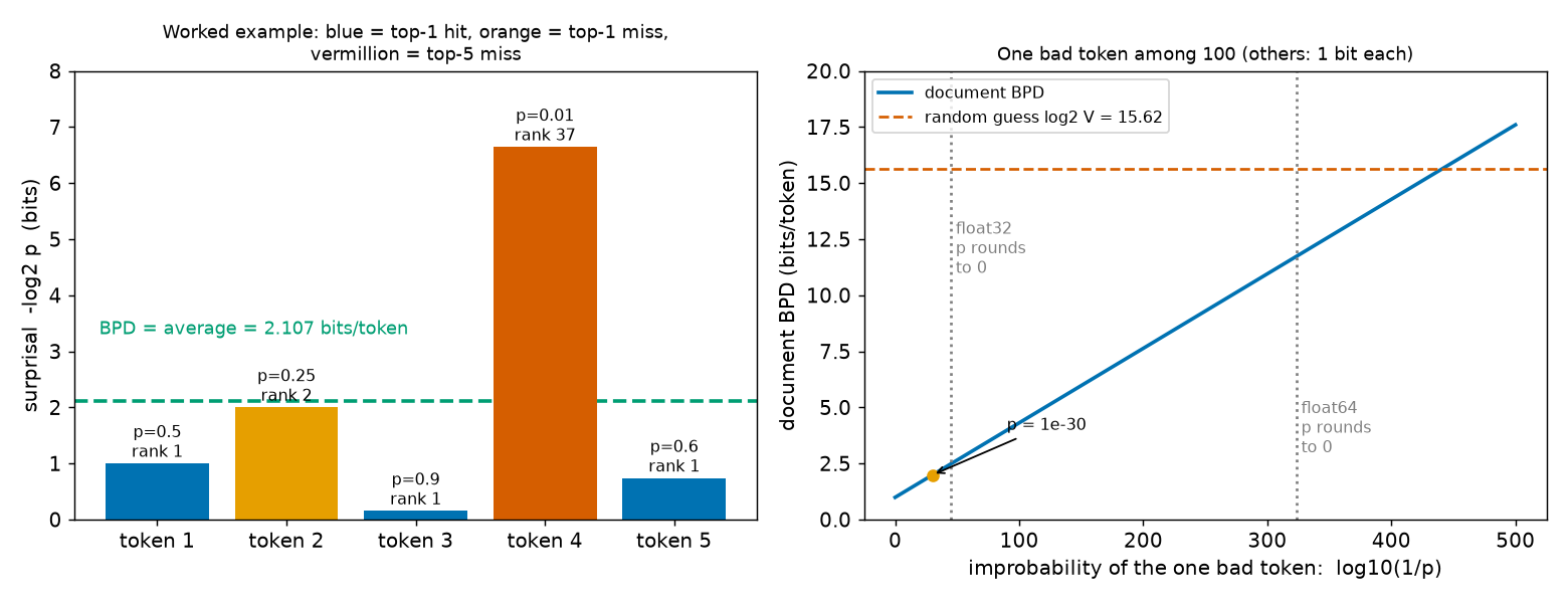
Step 2 — the document's scores¶
- Likelihood: \(p(X) = 0.5 \times 0.25 \times 0.9 \times 0.01 \times 0.6 = 0.000675 = 2^{-10.533}\).
- NLL: \(1.000 + 2.000 + 0.152 + 6.644 + 0.737 = 10.533\) bits \(= 7.301\) nats.
- BPD: \(10.533 / 5 = 2.107\) bits per token, which is \(2.107 \times \ln 2 = 1.460\) nats per token.
- Perplexity: \(2^{2.107} = e^{1.460} = 4.307\). The geometric mean of the five probabilities is \(0.2322 = 1/4.307\); their arithmetic mean is 0.4520.
- Top-1 error: the real token was not the top guess at positions 2 and 4, so \(2/5 = 0.4\).
- Top-5 error: only position 4 (rank 37) falls outside the top 5, so \(1/5 = 0.2\). The top-k error stays 0.2 up to \(k = 36\) and drops to 0.0 at \(k = 37\).
Token 4 alone contributes \(6.644/5 = 1.329\) of the 2.107 bits per token: 63.1 % of the document's BPD comes from one token in five. Its top-1 contribution is one miss, the same as the mild miss at position 2.
Step 3 — two documents, two averages¶
Document A has \(L = 2\) tokens and BPD 12 bits per token (say, a near-empty page that is hard to predict). Document B has \(L = 200\) tokens and BPD 3.
- Document-level average: \((12 + 3)/2 = 7.500\) bits per token.
- Token-level average: \((2 \times 12 + 200 \times 3)/202 = 3.0891\) bits per token.
Same model, same two documents, and the reported number changes by more than a factor of 2.
A larger illustration uses an invented corpus of 10,000 documents, with lengths drawn from a skewed (lognormal) distribution (mean 1117.1 tokens, close to OpenWebText's 1,128.1 from Chapter 4's script; median 674; from 14 to 22,113) and with the assumption that short documents are harder to predict.
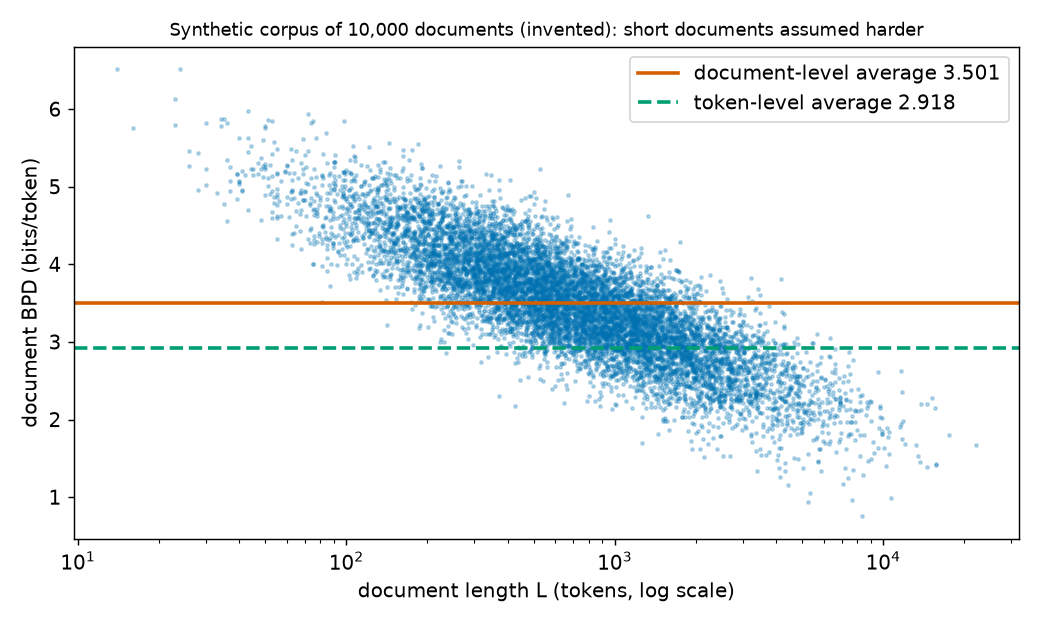
- With BPD falling with length: document-level 3.501, token-level 2.918, a difference of −0.583 bits per token.
- With the same BPD values assigned to lengths at random: document-level 3.501, token-level 3.503, a difference of +0.002.
The size of the gap depends entirely on how BPD and length are related in the real data, which the paper does not report. That is why erratum E28 matters.
Step 4 — one catastrophic token¶
Take a 100-token document in which 99 tokens have probability 0.5 (1 bit each).
- If the 100th token also has \(p = 0.5\): BPD \(= 1.000\).
- If it has \(p = 10^{-30}\): its surprisal is 99.658 bits, and BPD \(= (99 + 99.658)/100 = 1.987\). One token added 0.997 bits per token. The top-1 error, in contrast, can move by at most \(1/100 = 0.01\) because of one token.
- The document's BPD passes the random-guess level \(\log_2 V = 15.617\) once that single token's surprisal exceeds 1462.7 bits, that is, once \(p < 2^{-1462.7} = 10^{-440.3}\). Such probabilities are far too small for a computer to store as numbers, while a log-softmax can still produce log-probabilities that negative.
- In float32, softmax of the logits \([0, -110]\) gives the second token probability 0.0. Its surprisal is then infinite, and so is the document's BPD. Computed with log-softmax, the same token costs 110.0 nats \(= 158.70\) bits, and the BPD is 2.577.
Step 5 — the paper's random-guess column¶
SOURCE: GPT-2 tokenizer \(V = 50{,}257\). MY EXPLANATION The paper never prints this value (erratum E36; Chapter 3).
| Metric | Recomputed | Rounded to 2 decimals | Truncated | Table 1 prints |
|---|---|---|---|---|
| BPD, \(\log_2 V\) | 15.6170 | 15.62 | 15.61 | 15.62 |
| Top-1 error, \(1 - 1/V\) | 99.9980 % | 100.00 | 99.99 | 99.99 |
| Top-10 error, \(1 - 10/V\) | 99.9801 % | 99.98 | 99.98 | 99.98 |
| Top-100 error, \(1 - 100/V\) | 99.8010 % | 99.80 | 99.80 | 99.80 |
PAPER Table 1, p. 6 The printed values are those of the last column.
Paper erratum E21: the top-1 random-guess entry is truncated
PAPER Table 1, p. 6; Table 4, p. 14 The top-1 random-guess level is printed as 99.99.
MY EXPLANATION \(1 - 1/50{,}257 = 99.9980\,\%\) rounds to 100.00 %, not 99.99 %. The entry was truncated. The same column rounds \(\log_2 V = 15.6170\) up to 15.62 (truncation would give 15.61), so the table does not use one convention. No conclusion changes: every non-vacuous claim in the table has a margin far larger than 0.01 percentage points.
Step 6 — Table 2: what "Validation NLL" means¶
PAPER Table 2, p. 7 The paper reports, for the models with the best BPD bound:
| Model | Validation BPD | Validation NLL (paper) |
|---|---|---|
| SubLoRA | 10.53 | 7.29 |
| LoRA Only | 11.21 | 7.77 |
| Subspace Only | 13.85 | 9.60 |
| Original Model | 4.35 | 3.01 |
MY EXPLANATION Multiply each BPD by \(\ln 2 = 0.693147\):
| Model | BPD × ln 2 | Paper NLL | Difference | Perplexity \(2^{\mathrm{BPD}}\) |
|---|---|---|---|---|
| SubLoRA | 7.2988 | 7.29 | −0.0088 | 1,478.6 |
| LoRA Only | 7.7702 | 7.77 | −0.0002 | 2,368.9 |
| Subspace Only | 9.6001 | 9.60 | −0.0001 | 14,766.1 |
| Original Model | 3.0152 | 3.01 | −0.0052 | 20.4 |
All four agree to within 0.01. So "Validation NLL" is the same measurement as "Validation BPD", expressed in nats per token.
Paper erratum E27: the unit of 'Validation NLL' is not stated
PAPER Table 2, p. 7; §4.3, p. 5; Fig. 2, p. 5 Table 2's NLL row has no unit. Elsewhere the paper uses "NLL" as another name for BPD (§4.3; Figure 2's axis "NLL (BPD)").
MY EXPLANATION The table above shows NLL \(\approx\) BPD \(\times \ln 2\) for every model, so the row is in nats per token (erratum E27). A reader who took it for bits would conclude, wrongly, that the original GPT-2 scores 3.01 bits per token.
Paper erratum E46: Table 2's SubLoRA NLL is not the rounded value
PAPER Table 2, p. 7 SubLoRA: BPD 10.53, NLL 7.29.
MY EXPLANATION If both entries were rounded to two decimals, the true BPD would lie in \([10.525, 10.535)\), so the true NLL would lie in \([7.2954, 7.3023)\), which rounds to 7.30, never 7.29. The script tests every row: the SubLoRA row is consistent with truncating both numbers but not with rounding both; the other three rows are consistent with either. Together with erratum E21 (truncated) and Table 1's 15.62 (rounded), the paper's tables mix rounding conventions. The effect is at most 0.01 nats per token and changes no conclusion.
Paper erratum E47: is 'Validation BPD' measured on the smoothed or the unsmoothed model?
PAPER §4.3, p. 5; Table 2, p. 7 The bound certifies the smoothed model \(p_h\). Table 2 does not say whether its validation rows score \(p_h\) or the base model \(p_\theta\).
[SOURCE: authors' code, estimate_loss] The validation loss tracked in training is computed from the base
model's outputs, with no smoothing.
MY EXPLANATION If Table 2 reports that number, "bound 12.12 vs validation 10.53" compares two different models (smoothed vs unsmoothed) as well as two different averages (erratum E28). Smoothing changes BPD (Chapter 16), so the comparison is indicative only.
Perplexities. MY EXPLANATION The perplexity column makes the gaps visible. The best SubLoRA model's validation perplexity is about 1,478.6: it is as unsure as a uniform choice among roughly 1,500 tokens. The original GPT-2 is at 20.4, and random guessing at \(2^{\log_2 V} = 50{,}257\). The SubLoRA bound of 12.12 bits per token corresponds to a perplexity of 4,451.3.
Going deeper¶
Everything in this section is MY EXPLANATION.
The deeper blocks of this chapter sit next to the definitions they support:
- "Perplexity is an inverse geometric mean, and why that matters" — under Perplexity.
- "Proof of Gibbs' inequality, and BPD as an average cross-entropy" — under Cross-entropy and entropy.
- "How bits per token and top-k error constrain each other" — under Top-k prediction and top-k error.
- "Exactly how the two averages differ" — under From documents to a dataset.
- "The uniform predictor is the best worst-case predictor" — under Random-guess baselines.
One more block collects what this chapter means for the bound.
Going deeper: what each metric needs before a bound can use it
MY EXPLANATION Eq. (1) (Chapter 11) needs, for each document, one loss value \(R(h, X)\) that lies in a fixed interval of width \(\Delta\) known before the data are seen. The probability in the bound is over the random draw of the documents; \(h\) and \(\Delta\) are fixed.
| Metric | Per-document value | Interval | Width \(\Delta\) | Ready for Eq. (1)? |
|---|---|---|---|---|
| Top-k error | fraction of tokens outside the top k | \([0, 1]\) | 1 | yes |
| BPD of \(p_\theta\) | average log-loss | \([0, \infty)\) | none | no |
| BPD of \(p_h\) (smoothed) | average log-loss | a finite interval (Chapter 16) | finite | yes |
| Token-level average | not a per-document quantity | — | — | no |
Why the per-document average keeps the interval. If every per-token loss lies in \([a, a + \Delta]\), then their average over any number of tokens does too, because an average of numbers lies between their smallest and largest value. So a per-token cap becomes a per-document cap with the same width, whatever the document's length.
Why top-k error needs no smoothing. Each token contributes 0 or 1, so \(\Delta = 1\) from the start. Smoothing does not change it either. Smoothing replaces each probability \(p\) by \((1-\alpha)p + \alpha/V\) with \(0 < \alpha < 1\) (Chapter 16). This is the same increasing function applied to every token: if \(p_u > p_v\) then \((1-\alpha)p_u + \alpha/V > (1-\alpha)p_v + \alpha/V\), because \(1 - \alpha > 0\). The order of the tokens, and hence every top-k set, is unchanged.
What the bound is about. For BPD, the bounded quantity is \(R(h) = \mathbb E_X[\mathrm{BPD}(h, X)]\): the expected per-document average log-loss of the smoothed model on a fresh document. It is not a token-level cross-entropy, not a perplexity, and not a statement about the unsmoothed model.
Common misconceptions¶
- Misconception: NLL and BPD are different losses. — Actually: for one document they are the same quantity on different scales: NLL is the total, in bits or nats; BPD is the total in bits divided by the number of tokens. The paper's "Validation NLL" is BPD × ln 2 (nats per token): 4.35 bits per token becomes 3.0152 nats.
- Misconception: a low perplexity means the model is never badly wrong. — Actually: perplexity is \(2^{\text{BPD}}\), an inverse geometric mean of the probabilities. In the worked example one token of five supplies 63.1 % of the BPD; in the 100-token example, a single token at \(p = 10^{-30}\) adds 0.997 bits per token, and a single probability of exactly 0 makes perplexity infinite.
- Misconception: top-1 error and BPD always move together. — Actually: a top-1 hit can cost 14.617 bits (a nearly uniform model) and a top-1 miss only 1.322 bits. The only general links are weak: surprisal below \(\log_2(k+1)\) guarantees a top-k hit, so top-k error \(\le \mathrm{BPD}/\log_2(k+1)\).
- Misconception: averaging over tokens or over documents gives the same number. — Actually: they differ by \(\mathrm{Cov}(L, \mathrm{BPD})/\bar L\). Two documents of 2 and 200 tokens give 7.500 one way and 3.0891 the other. The bound uses the document-level average.
- Misconception: the random-guess level is the worst a model can do. — Actually: it is what a model that learned nothing achieves. A confident, wrong model can pay far more than \(\log_2 V\) bits per token; BPD has no upper limit.
- Misconception: softmax never outputs 0, so the log-loss is bounded in practice. — Actually: exact probabilities can be arbitrarily small, and float32 rounds a token with logit gap 110 to probability 0.0, making the document's BPD infinite. Prediction smoothing (Chapter 16) is what creates a bound.
Self-test¶
Q1. A model reads a 4-token document and gives the real tokens probabilities \(1/2, 1/4, 1/8, 1/16\); their ranks in the model's predictions are 1, 1, 3, 2. Compute the NLL (bits and nats), the BPD, the nats per token, the perplexity, and the top-1 and top-2 errors.
Answer
The surprisals are \(\log_2 2 = 1\), \(\log_2 4 = 2\), \(\log_2 8 = 3\) and \(\log_2 16 = 4\) bits, so the NLL is \(1 + 2 + 3 + 4 = 10\) bits \(= 10 \times \ln 2 = 6.931\) nats. BPD \(= 10/4 = 2.500\) bits per token \(= 1.733\) nats per token. Perplexity \(= 2^{2.5} = 5.657\). Top-1 error: tokens 3 and 4 are not ranked first, so \(2/4 = 0.50\). Top-2 error: only token 3 (rank 3) is outside the top 2, so \(1/4 = 0.25\) (output [Q1]). Note that token 4 (rank 2) has a higher surprisal than token 3 (rank 3): rank and surprisal are different things.
Q2. A colleague wants to report the bound's empirical risk by pooling all tokens of the 10,000 subsampled documents and dividing the total NLL by the total number of tokens. Why is this the wrong average for the paper's bound, and in which direction would it typically move the number if long documents are easier to predict?
Answer
The bound treats each document as one independent example with one loss \(R(h, X)\) in a fixed interval; its expected risk is \(\mathbb E_X[\mathrm{BPD}(h, X)]\), in which every document weighs the same. The empirical risk that estimates it must therefore be the document-level average \(\frac1n\sum_j \mathrm{BPD}(h, X_j)\). Pooling the tokens gives a length-weighted average, a ratio of two random sums that the Hoeffding argument does not cover and that converges to a different number, \(\mathbb E[L\,b]/\mathbb E[L]\). The two differ by \(\mathrm{Cov}(L, \mathrm{BPD})/\bar L\). If long documents have lower BPD, the covariance is negative and the pooled number is lower — in the synthetic corpus, 2.918 instead of 3.501 bits per token — so the reported "bound" would be too optimistic.
Q3. Table 2 lists the original GPT-2's Validation NLL as 3.01 and the random-guess BPD as 15.62. A reader says: "so GPT-2 is \(15.62/3.01 = 5.2\) times better than guessing." What is wrong, and what is a fair comparison?
Answer
The two numbers are in different units. 3.01 is in nats per token (erratum E27); in bits it is \(3.01/\ln 2 = 4.343\), matching the Validation BPD of 4.35. The fair ratio in bits per token is \(15.62/4.35 = 3.59\). Ratios of log-losses are not very meaningful anyway, because each bit halves the effective number of choices. In perplexity terms, guessing is a uniform choice among \(V = 50{,}257\) tokens while GPT-2 is as unsure as a choice among \(2^{4.35} = 20.4\): \(V/2^{4.35} = 2{,}464\) times fewer effective options. Also remember erratum E28: the validation average may be token-level, while the bound's risk is document-level.
Code for this chapter¶
Run it from the project root:
.venv/Scripts/python explainer/code/ch06_metrics.py
Source: ch06_metrics.py
"""Chapter 6 demo: measuring a language model (ch06_metrics.py).

Reproduces / checks:
  * the worked example of Chapter 6: NLL (bits and nats), BPD, perplexity and top-k errors of a 5-token
    document whose next-token distributions are written out in full over a toy vocabulary of 100 tokens;
  * document-level vs token-level averages (two documents; a synthetic corpus of 10,000 documents) and the
    identity  token-level - document-level = Cov(L, BPD) / mean(L);
  * the unbounded log-loss: one token of probability 1e-30 in a 100-token document; float32 underflow;
  * the paper's random-guess column (Table 1, p. 6): log2 V = 15.62 and 1 - k/V for k = 1, 10, 100 (erratum E21);
  * Table 2 (p. 7): Validation NLL = Validation BPD x ln 2, i.e. nats per token (erratum E27), with a rounding
    audit, and the perplexities 2^BPD;
  * cross-entropy >= entropy on a toy distribution (exact and Monte Carlo);
  * surprisal < log2(k+1) bits  =>  true token is in the top k; document top-k error <= BPD / log2(k+1).
V = 50,257 comes from the GPT-2 tokenizer (never printed in the paper; erratum E36).
"""
import sys
import math
from pathlib import Path

import numpy as np
import matplotlib
matplotlib.use("Agg")
import matplotlib.pyplot as plt

HERE = Path(__file__).resolve().parent
sys.path.insert(0, str(HERE))
import pacbound as pb  # noqa: E402

OUT_TXT = HERE / "outputs" / "ch06_metrics.txt"
FIG_DIR = HERE.parent / "docs" / "assets" / "fig"
OUT_TXT.parent.mkdir(parents=True, exist_ok=True)
FIG_DIR.mkdir(parents=True, exist_ok=True)

V = pb.V_GPT2          # [SOURCE: GPT-2 tokenizer] 50,257
LN2 = pb.LN2
BLUE, ORANGE, VERM, GREEN = "#0072B2", "#E69F00", "#D55E00", "#009E73"

lines = []


def say(s=""):
    print(s)
    lines.append(s)


def round2(x):
    return math.floor(x * 100 + 0.5) / 100


def trunc2(x):
    return math.floor(x * 100 + 1e-9) / 100


say("Chapter 6 demo: measuring a language model (ch06_metrics.py, seed 0)")

# ---------------------------------------------------------------------------
# [1] Worked example: a 5-token document, full distributions over 100 toy tokens
# ---------------------------------------------------------------------------
rng = np.random.default_rng(0)
V_TOY = 100
P_TRUE = [0.5, 0.25, 0.9, 0.01, 0.6]
RANK_TARGET = [1, 2, 1, 37, 1]
HIGH_MASS = {1: 0.0, 2: 0.6, 37: 0.72}   # mass shared by the tokens ranked above the true token


def build_dist(p, r):
    """A full next-token distribution over V_TOY tokens in which the true token has probability p and rank r."""
    true_id = int(rng.integers(V_TOY))
    others = [int(v) for v in rng.permutation(V_TOY) if v != true_id]
    hi_ids, lo_ids = others[: r - 1], others[r - 1:]
    a_mass = HIGH_MASS[r]
    b_mass = 1.0 - p - a_mass
    dist = np.zeros(V_TOY)
    dist[true_id] = p
    if hi_ids:
        w = 1 + 0.2 * (rng.random(len(hi_ids)) - 0.5)
        dist[hi_ids] = a_mass * w / w.sum()
    w = 1 + 0.2 * (rng.random(len(lo_ids)) - 0.5)
    dist[lo_ids] = b_mass * w / w.sum()
    assert abs(dist.sum() - 1) < 1e-12
    if hi_ids:
        assert dist[hi_ids].min() > p
    assert dist[lo_ids].max() < p
    return dist, true_id


dists, true_ids, ranks = [], [], []
for p, r in zip(P_TRUE, RANK_TARGET):
    d, t = build_dist(p, r)
    rank = 1 + int(np.sum(d > d[t]))                 # position of the true token in the descending order
    order = np.argsort(-d, kind="stable")
    assert rank == RANK_TARGET[len(ranks)]
    assert int(np.where(order == t)[0][0]) + 1 == rank
    dists.append(d)
    true_ids.append(t)
    ranks.append(rank)

p_arr = np.array(P_TRUE)
s_bits = -np.log2(p_arr)
s_nats = -np.log(p_arr)
L5 = len(p_arr)
ranks = np.array(ranks)

say("[1] Worked example: 5-token document; each next-token distribution written out over V_toy = 100 tokens")
say("    pos  p(true)  rank  surprisal (bits)  (nats)  top-1 miss  top-5 miss")
for i in range(L5):
    say(f"     {i+1}   {p_arr[i]:<6}  {ranks[i]:>4}       {s_bits[i]:7.3f}      {s_nats[i]:6.3f}       "
        f"{int(ranks[i] > 1)}           {int(ranks[i] > 5)}")
nll_bits, nll_nats = s_bits.sum(), s_nats.sum()
bpd = nll_bits / L5
nats_tok = nll_nats / L5
assert abs(nats_tok - bpd * LN2) < 1e-12
ppl = 2 ** bpd
assert abs(ppl - math.exp(nats_tok)) < 1e-9
geo = 2 ** (-bpd)
ari = p_arr.mean()
pX = float(np.prod(p_arr))
say(f"    p(X) = product = {pX:.6f} = 2^-{nll_bits:.3f};  NLL = {nll_bits:.3f} bits = {nll_nats:.3f} nats")
say(f"    BPD = {nll_bits:.3f}/5 = {bpd:.3f} bits/token = {nats_tok:.3f} nats/token;  perplexity 2^BPD = "
    f"e^(nats/token) = {ppl:.3f}")
say(f"    geometric mean of p = {geo:.4f} = 1/perplexity;  arithmetic mean of p = {ari:.4f} (1/that = {1/ari:.3f})")
topk = {k: float(np.mean(ranks > k)) for k in (1, 2, 5, 10, 36, 37)}
say("    top-k error of the document: " + ", ".join(f"k={k}: {v:.1f}" for k, v in topk.items()))
say(f"    token 4 alone contributes {s_bits[3]:.3f}/5 = {s_bits[3]/5:.3f} of the {bpd:.3f} bits/token "
    f"({100*s_bits[3]/nll_bits:.1f} %)")

# ---------------------------------------------------------------------------
# [2] Document-level vs token-level averages
# ---------------------------------------------------------------------------
say("[2] Averaging over documents")
LA, BA, LB, BB = 2, 12.0, 200, 3.0
doc_lvl = (BA + BB) / 2
tok_lvl = (LA * BA + LB * BB) / (LA + LB)
say(f"    doc A: L = {LA}, BPD = {BA};  doc B: L = {LB}, BPD = {BB}")
say(f"    document-level average = ({BA}+{BB})/2 = {doc_lvl:.3f};  token-level = ({LA}x{BA}+{LB}x{BB})/{LA+LB}"
    f" = {tok_lvl:.4f} bits/token")

rng_c = np.random.default_rng(0)
N_DOCS = 10_000
lengths = np.maximum(1, np.round(rng_c.lognormal(mean=math.log(680), sigma=1.0, size=N_DOCS))).astype(int)
noise = rng_c.normal(0, 0.4, size=N_DOCS)
bpd_corr = np.maximum(0.3, 3.2 + 0.6 * (math.log(1128) - np.log(lengths)) + noise)   # short docs harder (assumed)
bpd_ind = np.maximum(0.3, 3.2 + 0.6 * (math.log(1128) - np.log(rng_c.permutation(lengths))) + noise)


def both_avgs(b, L):
    doc = b.mean()
    tok = (b * L).sum() / L.sum()
    cov = np.mean((L - L.mean()) * (b - b.mean()))
    return doc, tok, cov / L.mean()


d1, t1, c1 = both_avgs(bpd_corr, lengths)
d2, t2, c2 = both_avgs(bpd_ind, lengths)
assert abs((t1 - d1) - c1) < 1e-10 and abs((t2 - d2) - c2) < 1e-10
say(f"    synthetic corpus (invented): {N_DOCS:,} documents, lengths lognormal, mean {lengths.mean():.1f} tokens,"
    f" median {np.median(lengths):.0f}, min {lengths.min()}, max {lengths.max():,}")
say(f"    BPD falls with length: document-level {d1:.3f}, token-level {t1:.3f}, difference {t1-d1:+.3f} bits/token")
say(f"    BPD unrelated to length: document-level {d2:.3f}, token-level {t2:.3f}, difference {t2-d2:+.3f}")
say(f"    identity token - doc = Cov(L, BPD)/mean(L) holds to {max(abs((t1-d1)-c1), abs((t2-d2)-c2)):.1e}")

# ---------------------------------------------------------------------------
# [3] Unbounded loss
# ---------------------------------------------------------------------------
say("[3] One bad token in a 100-token document (the other 99 tokens have p = 0.5, i.e. 1 bit each)")
s_bad = -math.log2(1e-30)
bpd_ok = (99 + 1.0) / 100
bpd_bad = (99 + s_bad) / 100
say(f"    bad token p = 0.5: BPD = {bpd_ok:.3f};  p = 1e-30: surprisal {s_bad:.3f} bits, BPD = {bpd_bad:.3f} "
    f"(+{s_bad/100:.3f} bits/token from one token); top-1 error moves by at most 1/100 = 0.01")
s_star = 100 * math.log2(V) - 99
say(f"    document BPD exceeds log2 V = {math.log2(V):.3f} once that token's surprisal exceeds {s_star:.1f} bits,"
    f" i.e. p < 2^-{s_star:.1f} = 10^-{s_star*math.log10(2):.1f}")
z = np.array([0.0, -110.0], dtype=np.float32)
e = np.exp(z - z.max())
p32 = e / e.sum()
with np.errstate(divide="ignore"):
    s32 = float(-np.log2(p32[1]))
bpd32 = (99 + s32) / 100
lsm = z - z.max() - np.log(np.sum(np.exp(z - z.max())))
s_lsm = float(-lsm[1]) / LN2
say(f"    float32 softmax of logits [0, -110]: p = {float(p32[1])} -> surprisal {s32} -> document BPD {bpd32}")
say(f"    same token via log-softmax: {float(-lsm[1]):.1f} nats = {s_lsm:.2f} bits -> document BPD "
    f"{(99 + s_lsm)/100:.3f}")
say(f"    smallest positive float32 = 2^-149 (surprisal cap 149 bits, 10^-{149*math.log10(2):.2f}); "
    f"float64 = 2^-1074 (10^-{1074*math.log10(2):.1f})")

# ---------------------------------------------------------------------------
# [4] Random-guess column of Table 1
# ---------------------------------------------------------------------------
say(f"[4] Random-guess baselines, V = {V:,} [SOURCE: GPT-2 tokenizer]")
lg = pb.random_guess_bpd(V)
say(f"    BPD: log2 V = {lg:.4f}; rounded {round2(lg):.2f}, truncated {trunc2(lg):.2f}; Table 1 prints 15.62 "
    f"(diff {15.62 - lg:+.4f})")
assert round2(lg) == 15.62
PAPER_TOPK = {1: 99.99, 10: 99.98, 100: 99.80}
for k, pv in PAPER_TOPK.items():
    x = 100 * pb.random_guess_topk_error(k, V)
    r2, t2_ = round2(x), trunc2(x)
    tag = "matches" if abs(r2 - pv) < 1e-9 else "ROUNDS TO %.2f; paper truncates (E21)" % r2
    say(f"    top-{k:<3} error 1 - k/V = {x:.4f} %; rounded {r2:.2f}, truncated {t2_:.2f}; paper {pv:.2f} -> {tag}")
    if k == 1:
        assert abs(t2_ - pv) < 1e-9 and abs(r2 - pv) > 1e-9
    else:
        assert abs(r2 - pv) < 1e-9
ranks_mc = rng.integers(1, V + 1, size=1_000_000)
mc = {k: float(np.mean(ranks_mc > k)) for k in (1, 10, 100)}
say("    uniformly random ranking, 1,000,000 simulated tokens: error " +
    ", ".join(f"top-{k} {100*v:.4f} %" for k, v in mc.items()))
V2 = 1000
q_model = rng.dirichlet(0.1 * np.ones(V2))
q_model = (q_model + 1e-12) / (q_model + 1e-12).sum()
ce_uniform_text = float(np.mean(-np.log2(q_model)))
say(f"    text drawn uniformly from {V2} tokens, some trained-looking model p: cross-entropy {ce_uniform_text:.3f}"
    f" bits >= log2 {V2} = {math.log2(V2):.3f}; its top-k error is exactly 1 - k/{V2}")
assert ce_uniform_text >= math.log2(V2)

# ---------------------------------------------------------------------------
# [5] Table 2: Validation NLL vs Validation BPD
# ---------------------------------------------------------------------------
say("[5] Table 2 (p. 7): Validation NLL vs Validation BPD x ln 2  (so NLL is in nats per token)")
TABLE2 = [("SubLoRA", 10.53, 7.29), ("LoRA Only", 11.21, 7.77), ("Subspace Only", 13.85, 9.60),
          ("Original Model", 4.35, 3.01)]
say("    model           BPD    BPDxln2   paper NLL   diff     round-consistent  trunc-consistent  perplexity 2^BPD")
for name, b, nl in TABLE2:
    conv = b * LN2
    diff = nl - conv
    assert abs(diff) <= 0.01
    # is there a true BPD that rounds to b and whose x ln2 rounds to nl?
    lo_r, hi_r = (b - 0.005) * LN2, (b + 0.005) * LN2
    rc = max(lo_r, nl - 0.005) < min(hi_r, nl + 0.005)
    lo_t, hi_t = b * LN2, (b + 0.01) * LN2
    tc = max(lo_t, nl) < min(hi_t, nl + 0.01)
    say(f"    {name:<15} {b:5.2f}   {conv:7.4f}   {nl:7.2f}   {diff:+.4f}   {str(rc):<16}  {str(tc):<16}  {2**b:,.1f}")
say(f"    bound 12.12 bits/token -> perplexity {2**12.12:,.1f};  random guess 2^log2 V = {2**lg:,.1f} = V")
say(f"    Original Model: 3.01 nats = {3.01/LN2:.3f} bits; V / 2^4.35 = {V/2**4.35:,.0f};  "
    f"15.62/4.35 = {15.62/4.35:.2f}")

# ---------------------------------------------------------------------------
# [6] Cross-entropy and entropy
# ---------------------------------------------------------------------------
say("[6] Cross-entropy H(q,p) = sum_v q(v) log2(1/p(v)) and entropy H(q) = H(q,q), 4 tokens")
q = np.array([0.5, 0.25, 0.125, 0.125])
models = {"p = q": q, "p uniform": np.full(4, 0.25), "p = (0.7,0.1,0.1,0.1)": np.array([0.7, 0.1, 0.1, 0.1])}
samples = rng.choice(4, size=200_000, p=q)
for name, pm in models.items():
    ce = float(np.sum(q * -np.log2(pm)))
    mc_ce = float(np.mean(-np.log2(pm[samples])))
    say(f"    {name:<22} H(q,p) = {ce:.4f} bits  (Monte Carlo, 200,000 tokens: {mc_ce:.4f});  "
        f"H(q,p) - H(q) = {ce - 1.75:.4f}")
    assert ce >= 1.75 - 1e-12

# ---------------------------------------------------------------------------
# [7] How surprisal and top-k constrain each other
# ---------------------------------------------------------------------------
say("[7] Surprisal vs top-k on 8,000 random distributions over 1,000 tokens (Dirichlet 0.1)")
N_TR, V3 = 8000, 1000
D = rng.dirichlet(0.1 * np.ones(V3), size=N_TR)
D = (D + 1e-12) / (D + 1e-12).sum(axis=1, keepdims=True)
from_model = rng.random(N_TR) < 0.5
tid = np.where(from_model, [rng.choice(V3, p=row) for row in D], rng.integers(V3, size=N_TR))
pt = D[np.arange(N_TR), tid]
surp = -np.log2(pt)
worst_rank = np.sum(D >= pt[:, None], axis=1)        # rank when every tie is broken against the true token
best_rank = 1 + np.sum(D > pt[:, None], axis=1)
viol = {}
for k in (1, 5, 10, 100):
    viol[k] = int(np.sum((surp < math.log2(k + 1)) & (worst_rank > k)))
    assert viol[k] == 0
say("    cases with surprisal < log2(k+1) but true token outside top k: " +
    ", ".join(f"k={k}: {v}" for k, v in viol.items()))
max_s_top1 = float(surp[best_rank == 1].max())
assert max_s_top1 <= math.log2(V3) + 1e-9
say(f"    largest surprisal of a top-1-correct token: {max_s_top1:.3f} bits <= log2 1000 = {math.log2(V3):.3f}")
DOC = 40
docs_s = surp[: (N_TR // DOC) * DOC].reshape(-1, DOC)
docs_r = worst_rank[: (N_TR // DOC) * DOC].reshape(-1, DOC)
mk_viol = 0
for k in (1, 5, 10, 100):
    mk_viol += int(np.sum((docs_r > k).mean(axis=1) > docs_s.mean(axis=1) / math.log2(k + 1) + 1e-12))
assert mk_viol == 0
say(f"    {N_TR // DOC} documents of {DOC} tokens: top-k error <= BPD/log2(k+1) violated {mk_viol} times "
    f"(k = 1, 5, 10, 100)")
near_unif = math.log2((V + 1) / 2)
say(f"    GPT-2 extremes: top-1 correct with p = 2/(V+1), others 1/(V+1): {near_unif:.3f} bits;  "
    f"top-1 wrong with p = 0.4 vs 0.6: {-math.log2(0.4):.3f} bits")

# ---------------------------------------------------------------------------
# [Q1] Self-test numbers
# ---------------------------------------------------------------------------
pq = np.array([1 / 2, 1 / 4, 1 / 8, 1 / 16])
rq = np.array([1, 1, 3, 2])
nb = float(np.sum(-np.log2(pq)))
say(f"[Q1] p = (1/2, 1/4, 1/8, 1/16), ranks (1, 1, 3, 2): NLL {nb:.0f} bits = {nb*LN2:.3f} nats; "
    f"BPD {nb/4:.3f}; {nb*LN2/4:.3f} nats/token; perplexity {2**(nb/4):.3f}; top-1 error "
    f"{np.mean(rq > 1):.2f}; top-2 error {np.mean(rq > 2):.2f}")

# ---------------------------------------------------------------------------
# Figures
# ---------------------------------------------------------------------------
plt.rcParams.update({"font.size": 11})
fig, (ax1, ax2) = plt.subplots(1, 2, figsize=(12, 4.6))
cols = [BLUE if r == 1 else (ORANGE if r <= 5 else VERM) for r in ranks]
ax1.bar(np.arange(1, 6), s_bits, color=cols)
for i in range(L5):
    ax1.text(i + 1, s_bits[i] + 0.12, f"p={P_TRUE[i]}\nrank {ranks[i]}", ha="center", fontsize=9)
ax1.axhline(bpd, color=GREEN, ls="--", lw=2, zorder=0)
ax1.text(0.55, bpd + 1.2, f"BPD = average = {bpd:.3f} bits/token", color=GREEN, fontsize=10)
ax1.set_xticks(range(1, 6))
ax1.set_xticklabels([f"token {i}" for i in range(1, 6)])
ax1.set_ylabel("surprisal  -log2 p  (bits)")
ax1.set_ylim(0, 8)
ax1.set_title("Worked example: blue = top-1 hit, orange = top-1 miss,\nvermillion = top-5 miss", fontsize=10)

xs = np.linspace(0, 500, 501)
ax2.plot(xs, (99 + xs * math.log2(10)) / 100, color=BLUE, lw=2, label="document BPD")
ax2.axhline(lg, color=VERM, ls="--", label=f"random guess log2 V = {lg:.2f}")
ax2.axvline(149 * math.log10(2), color="grey", ls=":")
ax2.axvline(1074 * math.log10(2), color="grey", ls=":")
ax2.text(149 * math.log10(2) + 4, 11, "float32\np rounds\nto 0", fontsize=9, color="grey")
ax2.text(1074 * math.log10(2) + 4, 3, "float64\np rounds\nto 0", fontsize=9, color="grey")
ax2.plot([30], [bpd_bad], "o", color=ORANGE)
ax2.annotate("p = 1e-30", (30, bpd_bad), xytext=(90, 4), arrowprops=dict(arrowstyle="->"), fontsize=9)
ax2.set_xlabel("improbability of the one bad token:  log10(1/p)")
ax2.set_ylabel("document BPD (bits/token)")
ax2.set_title("One bad token among 100 (others: 1 bit each)", fontsize=10)
ax2.legend(loc="upper left", fontsize=9)
ax2.set_ylim(0, 20)
fig.tight_layout()
fig.savefig(FIG_DIR / "ch06_example.png", dpi=130)
plt.close(fig)

fig, ax = plt.subplots(figsize=(8, 4.8))
ax.scatter(lengths, bpd_corr, s=3, alpha=0.25, color=BLUE)
ax.axhline(d1, color=VERM, lw=2, label=f"document-level average {d1:.3f}")
ax.axhline(t1, color=GREEN, lw=2, ls="--", label=f"token-level average {t1:.3f}")
ax.set_xscale("log")
ax.set_xlabel("document length L (tokens, log scale)")
ax.set_ylabel("document BPD (bits/token)")
ax.set_title("Synthetic corpus of 10,000 documents (invented): short documents assumed harder", fontsize=10)
ax.legend(loc="upper right")
fig.tight_layout()
fig.savefig(FIG_DIR / "ch06_averaging.png", dpi=130)
plt.close(fig)

say("figures: docs/assets/fig/ch06_example.png, docs/assets/fig/ch06_averaging.png. All assertions passed.")
OUT_TXT.write_text("\n".join(lines) + "\n", encoding="utf-8")
Output:
Chapter 6 demo: measuring a language model (ch06_metrics.py, seed 0)
[1] Worked example: 5-token document; each next-token distribution written out over V_toy = 100 tokens
    pos  p(true)  rank  surprisal (bits)  (nats)  top-1 miss  top-5 miss
     1   0.5        1         1.000       0.693       0           0
     2   0.25       2         2.000       1.386       1           0
     3   0.9        1         0.152       0.105       0           0
     4   0.01      37         6.644       4.605       1           1
     5   0.6        1         0.737       0.511       0           0
    p(X) = product = 0.000675 = 2^-10.533;  NLL = 10.533 bits = 7.301 nats
    BPD = 10.533/5 = 2.107 bits/token = 1.460 nats/token;  perplexity 2^BPD = e^(nats/token) = 4.307
    geometric mean of p = 0.2322 = 1/perplexity;  arithmetic mean of p = 0.4520 (1/that = 2.212)
    top-k error of the document: k=1: 0.4, k=2: 0.2, k=5: 0.2, k=10: 0.2, k=36: 0.2, k=37: 0.0
    token 4 alone contributes 6.644/5 = 1.329 of the 2.107 bits/token (63.1 %)
[2] Averaging over documents
    doc A: L = 2, BPD = 12.0;  doc B: L = 200, BPD = 3.0
    document-level average = (12.0+3.0)/2 = 7.500;  token-level = (2x12.0+200x3.0)/202 = 3.0891 bits/token
    synthetic corpus (invented): 10,000 documents, lengths lognormal, mean 1117.1 tokens, median 674, min 14, max 22,113
    BPD falls with length: document-level 3.501, token-level 2.918, difference -0.583 bits/token
    BPD unrelated to length: document-level 3.501, token-level 3.503, difference +0.002
    identity token - doc = Cov(L, BPD)/mean(L) holds to 9.2e-16
[3] One bad token in a 100-token document (the other 99 tokens have p = 0.5, i.e. 1 bit each)
    bad token p = 0.5: BPD = 1.000;  p = 1e-30: surprisal 99.658 bits, BPD = 1.987 (+0.997 bits/token from one token); top-1 error moves by at most 1/100 = 0.01
    document BPD exceeds log2 V = 15.617 once that token's surprisal exceeds 1462.7 bits, i.e. p < 2^-1462.7 = 10^-440.3
    float32 softmax of logits [0, -110]: p = 0.0 -> surprisal inf -> document BPD inf
    same token via log-softmax: 110.0 nats = 158.70 bits -> document BPD 2.577
    smallest positive float32 = 2^-149 (surprisal cap 149 bits, 10^-44.85); float64 = 2^-1074 (10^-323.3)
[4] Random-guess baselines, V = 50,257 [SOURCE: GPT-2 tokenizer]
    BPD: log2 V = 15.6170; rounded 15.62, truncated 15.61; Table 1 prints 15.62 (diff +0.0030)
    top-1   error 1 - k/V = 99.9980 %; rounded 100.00, truncated 99.99; paper 99.99 -> ROUNDS TO 100.00; paper truncates (E21)
    top-10  error 1 - k/V = 99.9801 %; rounded 99.98, truncated 99.98; paper 99.98 -> matches
    top-100 error 1 - k/V = 99.8010 %; rounded 99.80, truncated 99.80; paper 99.80 -> matches
    uniformly random ranking, 1,000,000 simulated tokens: error top-1 99.9973 %, top-10 99.9797 %, top-100 99.8000 %
    text drawn uniformly from 1000 tokens, some trained-looking model p: cross-entropy 19.968 bits >= log2 1000 = 9.966; its top-k error is exactly 1 - k/1000
[5] Table 2 (p. 7): Validation NLL vs Validation BPD x ln 2  (so NLL is in nats per token)
    model           BPD    BPDxln2   paper NLL   diff     round-consistent  trunc-consistent  perplexity 2^BPD
    SubLoRA         10.53    7.2988      7.29   -0.0088   False             True              1,478.6
    LoRA Only       11.21    7.7702      7.77   -0.0002   True              True              2,368.9
    Subspace Only   13.85    9.6001      9.60   -0.0001   True              True              14,766.1
    Original Model   4.35    3.0152      3.01   -0.0052   True              True              20.4
    bound 12.12 bits/token -> perplexity 4,451.3;  random guess 2^log2 V = 50,257.0 = V
    Original Model: 3.01 nats = 4.343 bits; V / 2^4.35 = 2,464;  15.62/4.35 = 3.59
[6] Cross-entropy H(q,p) = sum_v q(v) log2(1/p(v)) and entropy H(q) = H(q,q), 4 tokens
    p = q                  H(q,p) = 1.7500 bits  (Monte Carlo, 200,000 tokens: 1.7505);  H(q,p) - H(q) = 0.0000
    p uniform              H(q,p) = 2.0000 bits  (Monte Carlo, 200,000 tokens: 2.0000);  H(q,p) - H(q) = 0.2500
    p = (0.7,0.1,0.1,0.1)  H(q,p) = 1.9183 bits  (Monte Carlo, 200,000 tokens: 1.9199);  H(q,p) - H(q) = 0.1683
[7] Surprisal vs top-k on 8,000 random distributions over 1,000 tokens (Dirichlet 0.1)
    cases with surprisal < log2(k+1) but true token outside top k: k=1: 0, k=5: 0, k=10: 0, k=100: 0
    largest surprisal of a top-1-correct token: 5.382 bits <= log2 1000 = 9.966
    200 documents of 40 tokens: top-k error <= BPD/log2(k+1) violated 0 times (k = 1, 5, 10, 100)
    GPT-2 extremes: top-1 correct with p = 2/(V+1), others 1/(V+1): 14.617 bits;  top-1 wrong with p = 0.4 vs 0.6: 1.322 bits
[Q1] p = (1/2, 1/4, 1/8, 1/16), ranks (1, 1, 3, 2): NLL 10 bits = 6.931 nats; BPD 2.500; 1.733 nats/token; perplexity 5.657; top-1 error 0.50; top-2 error 0.25
figures: docs/assets/fig/ch06_example.png, docs/assets/fig/ch06_averaging.png. All assertions passed.