24. The pipeline: §4, §6.1, Algorithm 1, Appendices C and E¶

Where this fits

Prerequisites: Chapter 14 (compressed size, the "+2 log₂ C" header, hyperparameter bits), Chapter 15 (documents as the i.i.d. units), Chapter 16 (prediction smoothing, \(\Delta(\alpha)\)), Chapter 17 (the subsampling bound, Eq. 3), Chapter 18 and Chapter 19 (random subspaces, LoRA), Chapter 20 (SubLoRA), Chapter 21 (quantization, codebook, k-means, straight-through estimator), Chapter 22 (arithmetic coding, header cost). Used later by: Chapter 25, Chapter 26, Chapter 28, Chapter 29. Purpose: put every part built so far into the order the paper runs them, trace one real model through Algorithm 1 down to Table 1's 12.12 bits per token, and check that the paper's description of the pipeline matches what was computed.

The problem this chapter solves¶

Everything in this section is MY EXPLANATION unless tagged.

Chapters 14 to 22 each built one part of the machine. One chapter proved the bound. Another made the loss bounded. Another made the model small. Another turned the small model into a short bit string.

A machine is more than its parts. The parts must be run in the right order. Each part must hand the next one a quantity in the right unit. And every choice made along the way must be paid for somewhere in the bound.

PAPER §6.1, pp. 6–7; App. C, p. 15; App. E, pp. 16–17 The paper describes this assembly in three places: a prose summary (§6.1), a short program written in plain-English-like code (Algorithm 1, Appendix C), and a list of settings (Appendix E).

This chapter does three jobs.

It maps every line of Algorithm 1 to the chapter that explains it.
It runs the best GPT-2-small model through Algorithm 1 with real numbers, line by line, and lands on the paper's 12.12 bits per token.
It audits the details the paper leaves loose: what the hyperparameter bits pay for, what Algorithm 1 forgets to pass along, and a formula for long documents (Eq. 9) that does not do what its sentence says.

Intuition (and where the analogy breaks)¶

Everything in this section is MY EXPLANATION.

Think of a bakery that wants to print a guarantee on its cookie boxes: "the average cookie scores at least so well". It works like an assembly line with five stations.

Bake. Develop a recipe by trial and error on the bakery's huge stock of past orders (training).
Round. Round every quantity in the recipe to a few allowed amounts, then re-tune the recipe knowing it will be rounded (quantization).
Write the card. Write the rounded recipe on a card as short as possible. The longer the card, the less the guarantee is worth (compressed size, priced through the prior).
Taste. Taste 10,000 cookies picked at random from 8 million, instead of all of them (subsampling).
Certify. Print: taste score + a penalty for the card length + a penalty for having tasted only a sample.

The guarantee is honest only if every station plays by the rules. The card must be written in a code agreed before baking. The cookies must be picked at random. And any choice made by looking at the tasting results must be paid for.

Where it breaks.

The "card" is not a description of how the recipe was found. It describes only the finished recipe. Settings that steered the trial and error (how fast to adjust, how long to bake) never need to appear on the card. In the paper this means the learning rate need not be paid for, although the paper pays for it anyway.
In a bakery the tasting does not change the recipe. In the paper it does a little: the smoothing weight \(\alpha\) and the subspace dimension \(d\) are picked by comparing bounds computed on the same 10,000 documents. That is a hidden extra choice (erratum E07, previewed below).
A cookie guarantee is about cookies from the same bakery. The paper's guarantee is likewise only about documents drawn like the OpenWebText training documents, not about text in general (Chapter 15).

What the paper says, precisely¶

§4: the three improvements¶

PAPER §4, p. 4 The methods section opens by listing three ways in which the paper extends earlier compression bounds:

a simple nonlinear parameterization of the network that compresses better and scales further than a purely linear random subspace;
bounds that cope with the negative log-likelihood, a continuous and unbounded loss;
bounds that stay valid when the training loss is measured on a small random subsample only.

MY EXPLANATION In this explainer: (1) is SubLoRA (Chapter 20, built on Chapter 18 and Chapter 19); (2) is the pair "documents as the i.i.d. unit" (Chapter 15) plus prediction smoothing (Chapter 16); (3) is the subsampling bound, Eq. (3) (Chapter 17). The base result they all plug into is the compression bound of Chapter 14.

§6.1: the end-to-end pipeline¶

MY EXPLANATION An end-to-end pipeline is the complete sequence of steps from raw data to the final reported number, with the output of each step feeding the next.

PAPER §6.1, pp. 6–7 The paper's pipeline, paraphrased:

Train GPT-style networks through the SubLoRA parameterization, Eq. (4), for several values of the subspace dimension \(d\) and two values of the LoRA rank \(r\).
Near the end of training, run extra steps of quantization-aware training with a small number of levels.
Write the trained vector \(w\) in this quantized form and arithmetic-code it. The length of the code is the compressed size. Add the bits needed to say which \(d\), \(r\), \(\alpha\), learning rate and number of levels were used.
Compute each token's log-probability and top-k predictions on \(n = 10{,}000\) training documents.
Evaluate Eq. (3) as a function of \(\alpha\) and keep the best \(\alpha\) for each model.
Compare the choices of \(d\) and keep the one with the best bound.

MY EXPLANATION Steps 1, 5 and 6 together are a grid search: try every combination of a few listed values of each hyperparameter and keep the best result. The list of combinations, fixed before training, is the hyperparameter grid. Appendix E gives the lists (below).

Algorithm 1, line by line¶

MY EXPLANATION Pseudo-code is a program written for human readers: it names the steps and their inputs and outputs in a programming-like layout but cannot be run as it stands. A function in pseudo-code is a named step that takes inputs and returns an output. Algorithm 1 is the paper's pseudo-code for one bound computation.

PAPER App. C, Algorithm 1, p. 15 The table paraphrases each line. The column "in our notation" and the chapter column are MY EXPLANATION. Names in capitals are the paper's function names.

Line	What the line does (paraphrased)	In our notation	Explained in
1	Inputs: the network, the \(m\) training documents, the \(n\) subsampled documents, the number of quantization levels (the paper calls it \(C\)), \(d\), \(r\), \(\alpha\), confidence \(1-\delta\)	\(\{X_j\}_{j=1}^m\), \(\{X_{\sigma(i)}\}_{i=1}^n\), \(L_q\), \(d\), \(r\), \(\alpha\), \(\delta\)	Ch. 15, 17
2	Header of `COMPUTE_BOUND`; its argument list has an \(L\) where line 1 has \(C\)	—	erratum E17
3	`TRAIN_SUBLORA`: train \(w\) with dimension \(d\) and rank \(r\) on the training documents	\(\theta=\theta_0+\mathrm{LoRA}(Pw)\), Eq. (4)	Ch. 20
4	`TRAIN_QUANTIZE`: turn \(w\) into a quantized vector \(\hat w\) with \(L_q\) levels	\(\hat w\)	Ch. 21
5	Smoothed empirical risk of the quantized model on the subsample	\(\hat{\hat R}(\hat h)\) with \(p_h=(1-\alpha)p_\theta+\alpha/V\)	Ch. 15, 16, 17
6	The price of the hypothesis is set to the compressed size	\(\ln\frac{1}{P(\hat h)}\)	Ch. 12, 13, 14
7	Return the finite-hypothesis bound with subsampling	Eq. (3)	Ch. 17
9–10	`TRAIN_QUANTIZE` starts the levels \(c\) with k-means	codebook \(c=(c_1,\dots,c_{L_q})\)	Ch. 21
11–13	For a number of epochs: one gradient step on \(c\) and one on \(w\), step size \(\rho\)	quantization-aware training	Ch. 7, 21
14	Return \(\hat w\)	\(\hat w_i\) = the level nearest to \(w_i\)	Ch. 21
16–17	`GET_COMPRESSED_SIZE` lists the distinct values of \(\hat w\) and how often each occurs	codebook, counts	Ch. 21, 22
18	Arithmetic-code \(\hat w\) with those frequencies	message of about \(d\,H(\hat p)\) bits	Ch. 22
19	Add the bits for the hyperparameter search	\(+\log_2 N\) bits	Ch. 14, this chapter
20	Return message size \(+\,2\times\log(\text{message size})\)	\(C+2\log_2 C\) bits	Ch. 12, 14

PAPER App. C, p. 15 The text under the algorithm adds that \(\hat w_i = c_q\) with \(q\) the index of the level nearest to \(w_i\), that the levels are learned together with \(w\) after a k-means start, and that the bound is computed for several values of \(r\), \(d\), the number of levels and \(\alpha\), paying extra bits for each, with the lowest bound reported.

MY EXPLANATION So Algorithm 1 describes one point of the search. The loop over the grid and the choice of the best result happen outside the algorithm, in the last sentence of Appendix C.

Paper erratum E17: Algorithm 1's arguments and symbols do not line up

PAPER App. C, Algorithm 1, p. 15 The function header takes an argument \(L\) that is not among the listed inputs (the inputs call the number of levels \(C\); erratum E16 lists the other uses of \(L\) and \(C\)). Line 7 passes neither \(\delta\) nor \(\alpha\) to GET_FINITE_HYPOTHESIS_BOUND, although Eq. (3) needs \(\delta\) and the width \(\Delta(\alpha)\). Line 12 differentiates through the nearest-level assignment, which has zero derivative almost everywhere; it needs the straight-through estimator (Chapter 21), which this paper does not describe. Line 20's "log" must be \(\log_2\) (next block).

Erratum E64 (extends E17). MY EXPLANATION Three more loose ends: TRAIN_QUANTIZE returns \(\hat w\) in line 14 but never computes it (lines 10–13 update only \(c\) and \(w\); the nearest-level step is in the prose below the algorithm); the step size \(\rho\), the loss \(\mathcal L(w,c)\) and quant_epochs are never defined; and line 6 stores a size in bits in a variable named \(\log 1/P(h)\), which Eq. (3) uses in nats. None of these changes a number if read as intended, but a reader implementing the pseudo-code literally would get line 6 wrong (see the next block).

Paper errata E02 and E52: two different logarithms hide in lines 6 and 20

PAPER App. C, Algorithm 1, lines 6 and 20, p. 15 Line 20 returns message size \(+\,2\times\log\)(message size), and line 6 calls that result \(\log 1/P(h)\).

MY EXPLANATION The message size is in bits, so line 20's log must be \(\log_2\): the header of a \(C\)-bit message costs about \(2\log_2 C\) bits (Chapter 12). [SOURCE: authors' code, quantize_model] The code uses np.log2 there. MY EXPLANATION The price in Eq. (3) must be in nats (its square root comes from \(e^{-2mt^2/\Delta^2}\) in Hoeffding's inequality), so line 6 must multiply by \(\ln 2\) (erratum E52, logged by Chapter 14). [SOURCE: authors' code, sublora_pipeline.py] The code does: divergence = (...) * np.log(2). The worked example below shows the size of each slip.

Hyperparameters are part of the hypothesis (Appendix C)¶

PAPER App. C, p. 15 When the bound is optimized over hyperparameters such as \(r\) and \(d\), the paper extends the hypothesis to \(h=(\theta,d,r)\). With the universal prior \(P(h)=2^{-K(h)}/Z\) it bounds \(K(h)\le K(\theta\mid d,r)+K(d)+K(r)\). If a hyperparameter is chosen from \(N\) values fixed in advance, naming the choice costs only \(\log_2 N\) bits, the same extra cost a separate union bound over the \(N\) choices would add.

MY EXPLANATION In words: to rebuild the model from the message, the decoder first needs to know which \(d\) and \(r\) were used, because the same string of quantized numbers means a different network for a different \(d\) or \(r\). Telling it costs \(\log_2 N\) bits per grid. Chapter 14 showed that this is a prior-weighted union bound in disguise and that the learning rate need not be paid for. The "Going deeper" block below proves the decomposition and says what the paper's inequality silently assumes.

Paper erratum E12: the decomposition holds only up to a constant, and only given the grid

PAPER App. C, p. 15 \(K(h)\le K(\theta\mid d,r)+K(d)+K(r)\) is written as an exact inequality.

MY EXPLANATION It holds up to an additive constant (the length of a fixed program that glues the three descriptions together; proof below). And "\(\log_2 N\) bits for \(d\)" is a bound on \(K(d\mid\text{grid})\), the complexity of \(d\) given the list of grid values, not on \(K(d)\) itself. Both gaps disappear if the prior is defined directly as (weight \(1/N\) for the grid point) × (length prior of the message), as in Chapter 12. Then the price is exactly \(C\ln 2+2\ln C+\ln N\) nats.

Appendix E: the experimental setup¶

PAPER App. E, pp. 16–17 The settings, paraphrased:

Code base and model. nanoGPT; a 124-million-parameter GPT-2-style model with 12 layers, 12 attention heads and embedding dimension 768 (Chapter 5).
Data. The training split of OpenWebText.
Training. Minibatches of 8 sequences of 1,024 tokens, sampled with replacement; AdamW with weight decay \(10^{-2}\) and \(\epsilon = 10^{-6}\) (the small constant that keeps Adam's division away from zero, Chapter 7); "no decay bias", which the paper does not explain (erratum E48; [SOURCE: authors' code, configure_optimizers] the flag exempts every one-dimensional tensor from weight decay).
LoRA. On the query and value matrices of every attention layer and on the linear head, with \(\alpha_{\text{LoRA}} = 32\) and LoRA dropout 0.1 (Chapter 19; the paper calls the scaling constant "LoRA alpha" and defines neither it nor the dropout, errata E16 and E55). §5 says only "the self-attention layer"; App. E is the precise statement (erratum E44).
Quantization and coding. Learned quantization of \(w\) as in Lotfi et al. (2022), then arithmetic coding with the empirical frequencies of the levels.
Grid for GPT-2 small. \(d\in\{5{,}000,\,10{,}000,\,25{,}000,\,50{,}000,\,100{,}000,\,200{,}000\}\), \(r\in\{1,4\}\), learning rate \(\in\{2\times10^{-4},\,5\times10^{-3},\,5\times10^{-5}\}\), \(\alpha\in\{0.0001,\,0.001,\,0.005,\,0.01,\,0.05,\,0.1,\,0.25,\,0.5\}\), \(L_q\in\{11,17\}\).
Model-size sweep. Eight shapes (layers, heads, embedding dimension) from (4, 4, 32) to (12, 12, 768), used for Figure 3 (Chapter 26).
Larger GPT-2 variants. 354M, 458M, 773M and 849M parameters (nominal labels; erratum E43), with \(r = 4\) and learning rate \(2\times10^{-4}\) fixed, \(d\in\{25{,}000,\,50{,}000\}\) and \(L_q\in\{11,17\}\).

MY EXPLANATION For GPT-2 small the hyperparameter grid therefore has \(6\times2\times3\times8\times2 = 576\) points (output [3]).

Paper erratum E40: Figure 2 shows values of d that are not in the grid

PAPER Fig. 2 left, p. 5; App. E, p. 16 Read exactly from the PDF, Fig. 2 (left) has points at \(d\) = 7,500 and 75,000 as well, which the Appendix E grid does not list.

MY EXPLANATION If eight values of \(d\) were searched, the grid has 768 points and the hyperparameter cost is \(\log_2 768 = 9.5850\) instead of \(\log_2 576 = 9.1699\) bits. For the best model the bound moves from 12.122225 to 12.122227 bits per token (output [3]). The issue is the completeness of the reported search, not the number.

Eq. (9): documents longer than the context¶

MY EXPLANATION A forward pass is one run of the network on one input window of at most \(L_{\text{ctx}}\) tokens. A causal transformer produces, in one forward pass, a next-token distribution for every position of the window, each using the tokens to its left inside the window (Chapter 5).

GPT-2 sees at most \(L_{\text{ctx}} = 1{,}024\) tokens. A document can be longer. So the "model" whose loss is bounded must include a rule for which tokens to show the network when it predicts token 1,500. Any fixed rule gives a valid autoregressive model (Chapter 4); the rule only has to be decided before the data are seen.

The simplest rule, "always show the last 1,024 tokens", costs one forward pass per token beyond 1,024. A sliding-window evaluation saves work: run one forward pass on a window, keep the predictions for the last few positions, then slide the window forward by a fixed number of tokens, the stride, and repeat.

PAPER App. E, p. 16 The paper writes \(x_{i:j}\) for the tokens \(x_i,\dots,x_j\) and \(f(x\mid z)\) for the network's probability of token \(x\) after context \(z\) of at most \(L\) tokens (here \(L = L_{\text{ctx}} = 1{,}024\)). For the first \(L\) tokens, \(p(x_i\mid x_{:i-1}) = f(x_i\mid x_{:i-1})\). For later tokens the text says the context is shifted "in chunks of size 100", and Eq. (9) defines

\[ p(x_i\mid x_{:i-1}) = f\big(x_i\mid x_{i-L':i-1}\big), \qquad L' = L - (i-L)\,\%\,100, \]

where \(\%\) is the remainder after division ("mod"). The stated purpose is to let batching shift the inputs by 100 tokens at a time instead of 1.

[SOURCE: authors' code, compute_bound_scores in bound_utils.py; sliding_window_size = 100 in the config] The code scores each sampled document starting from the end-of-text token in front of it. It runs one forward pass on the first 1,024 tokens, then windows that start at token 100, 200, 300, …, each 1,024 tokens long, keeping only the last 100 predictions of each window.

Paper erratum E15: Eq. (9) does not shift in chunks of 100

MY EXPLANATION Number the tokens so that \(x_0\) is the end-of-text token the code starts from and \(x_1, x_2, \dots\) are the scored tokens. Write \(j = i - L\) for how far token \(i\) lies beyond the first \(L\). The context of Eq. (9) as printed starts at token \(i - L' = j + (j \bmod 100)\). Script section [6] tabulates it:

token \(i\)	\(j\)	start, as printed	\(L'\), as printed	start, code	\(L'\), code
1,025	1	2	1,023	100	925
1,026	2	4	1,022	100	926
1,123	99	198	925	100	1,023
1,124	100	100	1,024	100	1,024
1,125	101	102	1,023	200	925

As printed, the start moves forward by two tokens per step for 99 steps and then jumps back by 98. Over \(j = 1\dots200\) it decreases twice; the code's start never decreases (output [6]). The printed rule is a legal model (every context has between 925 and 1,024 tokens), but it is not "shifting in chunks of 100", and it would need a separate forward pass for almost every token: 550 passes for a document of 2,048 scored tokens, against 12 for the stride-100 rule (output [6]).

The stride-100 rule of the code, written in the paper's form, is

\[ L' = L - 99 + \big((i - L - 1) \bmod 100\big), \qquad \text{start} = 100\left\lceil \frac{i-L}{100}\right\rceil . \]

The script re-implements the code's window arithmetic for a 6,000-token document and checks that this formula matches it at every token and that every token beyond \(L\) is scored exactly once (output [6]).

A note on an earlier draft of erratum E15. That draft suggested "\(L' = L - 100 + ((i-L) \bmod 100)\)". This variant differs from the code at the multiples of 100 (49 of 4,976 tokens in the test document), where it gives a 924-token context instead of 1,024. The errata page now gives the formula above.

Impact: none on validity. Whichever rule is used, it is fixed in advance and so belongs to the hypothesis for free; the bound certifies the model the code actually evaluated. The issue is that the paper's formula describes a different model from the one whose numbers it reports. If tokens were numbered from 1 without an \(x_0\), every index above shifts by one; the pattern does not change.

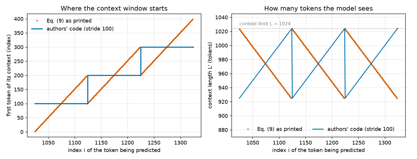
Context start and context length for the tokens just beyond the first 1,024, under Eq. (9) as printed and under the stride-100 rule of the authors' code

MY EXPLANATION Left: the printed rule's start (orange dots) climbs two tokens per step and falls back every 100 tokens; the code's start (blue steps) stays put for 100 tokens and then jumps forward by 100. Right: the number of tokens the network sees. Both stay at or below the context limit of 1,024.

What the authors' code adds¶

Code notes only; the code is used as evidence about what was run, never to fill in claims the paper does not make.

[SOURCE: authors' code, sample_single_document in utils.py; sublora_pipeline.py]

Each subsampled document is drawn uniformly at random from the list of training documents, independently each time (with replacement), and scored from its preceding end-of-text token. The loop stops after 10,000 documents.
\(m\) = num_docs = 8,009,762 and \(\delta\) = epsilon = 0.05 are the defaults; neither value appears in the paper (errata E31, E32).
The message length is message_len + 2 * np.log2(message_len), and message_len already includes 16 bits per codebook value and \(\lceil\log_2 d\rceil\) bits per count (get_message_len), so the code answers erratum E18 (below) with "yes, counted".
Hyperparameter bits: a configurable misc_extra_bits (7 in the released config) is added for every bound, and for the BPD bounds 8 more bits are added per \(\alpha\) inside the loop over \(\alpha\), so the 7th value (\(\alpha = 0.25\)) pays \(7 + 7\times8 = 63\) bits. MY EXPLANATION \(7 = \lceil\log_2(6\cdot2\cdot3\cdot2)\rceil\) would name one point of the \(d\times r\times\text{lr}\times L_q\) grid (output [3]); this reading is our guess. The total overpays, which only loosens the bound (by 0.000306 bits per token here, output [3]).
Training batches are random 1,024-token windows of the concatenated corpus (get_batch), not whole documents.
The released bound configuration is a template (paths read "TOADD") with max_quant_iters: 0 and use_kmeans: False. As shipped, it would skip quantization-aware training and quantize with equal-width bins instead of k-means. So the code does not tell us which settings produced the tables.
The sequence-level sampler (Appendix B) can reach only the first 8,617 of the 8,823,811 chunks, as found by Chapter 15 (its output [6]); this concerns the released code, not the paper's text.

Worked example with real numbers¶

Everything in this section is MY EXPLANATION unless tagged. All numbers are from ch24_pipeline.py (output sections in brackets).

The inputs¶

[PAPER Fig. 2, p. 5; read exactly from the PDF by fig_extract.py] The best GPT-2-small BPD model has \(d = 50{,}000\), smoothing weight \(\alpha = 0.25\), compressed size 16.5325 KB and subsampled smoothed empirical risk 10.5945 bits per token. Its \(r\), \(L_q\) and learning rate are not reported (erratum E33).

Other inputs (output [1]):

1 KB = 8,192 bits (erratum E35), so the compressed size is 135,434.26 bits.
\(m\) = 8,009,762 documents SOURCE: nanoGPT split / authors' code, \(n\) = 10,000 PAPER §6.1, \(\delta\) = 0.05 SOURCE: authors' code.
\(\Delta(0.25) = \log_2(1 + 0.75\cdot V/0.25) = 17.2020\) bits per token with \(V\) = 50,257 (Chapter 16).

Algorithm 1 in numbers¶

The table follows the lines in the order they compute (output [2]). The left value column has no hyperparameter bits; the right one pays \(\log_2 576\) bits in line 19.

Line	Quantity	No grid bits	With \(\log_2 576\)	Unit
18	arithmetic-coded message (incl. codebook and counts, see E18)	135,434.26	135,434.26	bits
19	+ hyperparameter bits	135,434.26	135,443.43	bits
20	+ header \(2\log_2(\cdot)\) (34.09 bits)	135,468.36	135,477.53	bits
6	price \(\ln\frac{1}{P(\hat h)}\) = bits × \(\ln 2\)	93,899.51	93,905.87	nats
5	\(\hat{\hat R}(\hat h)\), smoothed with \(\alpha = 0.25\)	10.5945	10.5945	bits/token
7	\(m\)-term \(\Delta\sqrt{(\ln\frac1{P}+\ln\frac{1}{s\delta})/(2m)}\)	1.31707	1.31711	bits/token
7	\(n\)-term \(\Delta\sqrt{\ln\frac{1}{(1-s)\delta}/(2n)}\)	0.21057	0.21057	bits/token
7	bound	12.122180	12.122225	bits/token

Here \(s = n/(n+m) = 0.001247\), \(\ln\frac{1}{s\delta} = 9.6828\) nats and \(\ln\frac{1}{(1-s)\delta} = 2.9970\) nats (output [2]), with \(\delta = 0.05\) and \(m\) = 8,009,762 taken from the authors' code [SOURCE], as listed above. PAPER Table 1, p. 6 The paper reports 12.12. Both columns round to it (difference +0.0022).

Two cross-checks against the paper's figures (output [2]):

Fig. 2 plots 12.1224 for this model; our value differs by 0.00019.
Fig. 1 (left) plots a complexity of 1.5278 for its best SubLoRA point; our two terms add to 1.5276.

Where the bound comes from: the empirical risk is 87.40 % of it, the \(m\)-term 10.86 % and the \(n\)-term 1.74 %. The uniform-guess level is \(\log_2 V = 15.6170\), so the bound sits 3.4949 bits per token below it (output [2]).

What the grid costs¶

Output [3] lists the bits for each way of counting the search, and the resulting bound:

What is paid for	Bits	Bound (bits/token)	Change
nothing	0	12.122180	—
App. E grid, \(N = 576\)	9.1699	12.122225	\(+4.46\times10^{-5}\)
8 values of \(d\) (E40), \(N = 768\)	9.5850	12.122227	\(+4.66\times10^{-5}\)
fixed-length index, \(\lceil\log_2 576\rceil\)	10	12.122229	\(+4.86\times10^{-5}\)
larger-model grid, \(N = 2\cdot2\cdot8 = 32\) (α grid assumed unchanged)	5	12.122204	\(+2.43\times10^{-5}\)
authors' code at \(\alpha = 0.25\)	63	12.122486	\(+3.06\times10^{-4}\)

Per hyperparameter, the 9.1699 bits split as \(d\): 2.5850, \(r\): 1, learning rate: 1.5850, \(\alpha\): 3, \(L_q\): 1 (output [3]). Each extra bit moves this bound by \(4.861\times10^{-6}\) bits per token. The "Going deeper" block below derives this number by hand.

The lesson: the hyperparameter bits are about 0.007 % of the price. They matter for honesty, not for the number.

What the loose ends cost¶

Output [4] prices the choices that Algorithm 1 leaves open:

Erratum E18 (below): if the codebook and counts were not already inside the 16.5325 KB, adding them would cost 352 bits (\(L_q = 11\)) or 544 bits (\(L_q = 17\)) (Chapter 22, its output [4]) and raise the bound by 0.0017 or 0.0026 bits per token.
Line 20 with \(\ln\) instead of \(\log_2\): the header would be 23.63 instead of 34.09 bits, and the bound would drop by \(5.09\times10^{-5}\). Wrong, but harmless in size.
Line 6 without the factor \(\ln 2\) (bits used as nats, errata E02 and E52): the bound would be 12.3870, 0.2649 higher. This is the only slip in the list that is visible at two decimals. It errs on the safe side.
Order of lines 19 and 20: Algorithm 1 adds the hyperparameter bits before the header; the code adds them after. The two differ by \(1.95\times10^{-4}\) bits.

Paper erratum E18: are the codebook and the counts in the message size?

PAPER App. C, Algorithm 1 lines 16–21, p. 15 Line 17 produces the codebook and the counts and line 18 passes them to the coder, but nothing adds their size, and the text does not say.

MY EXPLANATION The decoder cannot rebuild \(\hat w\) without them, so a valid bound must count them (Chapter 22). [SOURCE: authors' code, get_message_len] The code counts them. MY EXPLANATION Either way, the effect is at most 0.0026 bits per token (output [4]).

The hidden selection (preview of erratum E07)¶

Paper erratum E07: α and d are chosen on the same subsample that certifies them

PAPER §6.1, p. 7; App. C, p. 15 The bound is computed as a function of \(\alpha\) on the 10,000 subsampled documents and the best \(\alpha\) is kept; then the best \(d\) is kept.

MY EXPLANATION The hyperparameter bits enlarge the price in the \(m\)-term, which is a bound for all hypotheses at once. The \(n\)-term is a Hoeffding bound for one hypothesis fixed before the subsample was drawn. Choosing among \(N_{\text{sel}}\) candidates by their subsample scores needs \(\ln(N_{\text{sel}}/((1-s)\delta))\) in its place (Chapter 17 proves this and simulates the failure). For this model the repaired bound is 12.1857 (\(N_{\text{sel}} = 8\), \(\alpha\) only), 12.2304 (\(N_{\text{sel}} = 48\)) or 12.2836 (\(N_{\text{sel}} = 576\)) bits per token, against 12.1222 (output [5]). Still far below 15.6170, but not the number the stated theorem covers.

Going deeper¶

This hub collects the derivations behind the chapter. Everything below is MY EXPLANATION unless tagged.

Going deeper: what is fixed and what is random, station by station

Eq. (3) is a statement about probabilities, so its validity depends on the order in which things are chosen. Here is the pipeline sorted into "fixed before the data" and "random".

Fixed before any data are seen (they define the hypothesis space \(\mathcal H\) and the prior \(P\)): the architecture \(\mathcal A\); the seeds that generate \(\theta_0\), the LoRA initialization and the projector \(P\); the quantize-and-code scheme (how a message is decoded into \(\hat w\)); the hyperparameter grid; the rule for long documents (Eq. 9 or the stride-100 rule); \(\delta\), \(m\) and \(n\). A hypothesis is then a pair (grid point, message), and the prior is

\[ P(h) = \frac{1}{N}\cdot\frac{2^{-C(h)}}{C(h)^2}, \]

where \(N\) is the number of grid points and \(C(h)\) is the message length in bits. By the Kraft argument of Chapter 12, the second factor sums to at most \(\pi^2/6 - 1 < 1\) over all messages of one grid point (messages of length at least 2), and the first factor shares this among \(N\) points, so \(\sum_h P(h) \le 1\). Taking \(\ln\frac{1}{P(h)}\):

\[ \ln\frac{1}{P(h)} = \ln N + C(h)\ln 2 + 2\ln C(h) \quad\text{nats} = \big(C(h) + 2\log_2 C(h) + \log_2 N\big)\ln 2 . \]

The middle expression is lines 18–20 and 6 of Algorithm 1 (with lines 19 and 20 in the code's order).

Random, in this order:

The \(m\) training documents \(X_1,\dots,X_m\), i.i.d. from the document distribution (Chapter 15).
Training (lines 3–4). Any procedure is allowed: it may look at all documents, use random minibatches and its own random seed, and use any learning rate. Its output \(\hat h\) is a function of the documents and of training randomness that is independent of step 3.
The subsample indices \(\sigma(1),\dots,\sigma(n)\), uniform on \(\{1,\dots,m\}\), independent of everything above.
The value \(\hat{\hat R}(\hat h)\) (line 5) and the bound (line 7).

Why the bound holds for \(\hat h\). Chapter 17 proves two events. Event 1: for every \(h\in\mathcal H\) at once, \(R(h) \le \hat R(h) + m\text{-term}(h)\); it fails with probability at most \(s\delta\) over the draw of the documents. Because it covers every \(h\), it covers \(\hat h\) however training picked it. Event 2: with the documents (and therefore \(\hat h\)) held fixed, \(\hat R(\hat h) \le \hat{\hat R}(\hat h) + n\text{-term}\); it fails with probability at most \((1-s)\delta\) over the draw of \(\sigma\). The union bound gives both with probability at least \(1-\delta\).

Where the pipeline bends the rules. Event 2 needs \(\hat h\) fixed before \(\sigma\). Choosing \(\alpha\) and \(d\) by their Eq. (3) values on the subsample makes the final \(\hat h\) depend on \(\sigma\). That is erratum E07; the repair is a union over the \(N_{\text{sel}}\) candidates inside the \(n\)-term (output [5]).

Going deeper: proof that K(h) ≤ K(θ | d, r) + K(d) + K(r) + const

PAPER App. C, p. 15 states the inequality without the constant. MY EXPLANATION Here is the proof, using prefix Kolmogorov complexity on a fixed universal prefix machine \(U\) (Chapter 13).

Setup. Let \(p_d\) be a shortest self-delimiting program that makes \(U\) print \(d\); its length is \(K(d)\) bits. Let \(p_r\) be a shortest one for \(r\), length \(K(r)\). Let \(p_\theta\) be a shortest program that prints \(\theta\) when \(U\) is also given \((d,r)\) as side information, length \(K(\theta\mid d,r)\).

The glue program. Write a fixed program \(g\) that does the following: run the next self-delimiting program on the input and store its output as \(d\); run the next one and store its output as \(r\); run the next one with \((d,r)\) as side information and store its output as \(\theta\); print the triple \((\theta,d,r)\). This works because each of \(p_d\), \(p_r\), \(p_\theta\) is self-delimiting: \(U\) knows where each ends without an end marker, so the concatenation \(g\,p_d\,p_r\,p_\theta\) can be parsed.

Counting. The concatenation is a program for \(h=(\theta,d,r)\) of length \(|g| + K(d) + K(r) + K(\theta\mid d,r)\). \(K(h)\) is the length of the shortest such program, so

\[ K(h) \le K(\theta\mid d,r) + K(d) + K(r) + |g| . \]

The constant \(|g|\) depends on \(U\) but not on \(h\). The paper drops it (erratum E12).

The \(\log_2 N\) step. If \(d\) is one of \(N\) values listed in advance, a program that prints the list and then picks entry number \(k\) needs \(\lceil\log_2 N\rceil\) bits for \(k\) plus the bits that describe the list. The list is the same for every \(h\), so it can be built into \(U\)'s side information; then \(K(d\mid\text{grid}) \le \lceil\log_2 N\rceil + \text{const}\). Without that conditioning, \(K(d)\) is not bounded by \(\log_2 N\) (for example, \(K(200{,}000)\) has nothing to do with a six-item list).

The exact version. The prior of the previous block avoids all constants: it gives each grid point weight \(1/N\) directly, so the cost is exactly \(\log_2 N\) bits (not rounded up, since prior weights need not be powers of two). That is the version our numbers use.

What need not be paid for. Only what the decoder needs to rebuild the predictions: \(d\) and \(r\) (to interpret \(\hat w\)), \(\alpha\) (to smooth), and the codebook (sent in the message header). The learning rate, the number of training steps, the k-means start, \(\rho\) and quant_epochs affect which message training produces, not how a message is decoded. They are covered by the union over all messages already (Chapter 14). The paper's \(\log_2 3 = 1.5850\) bits for the learning rate (output [3]) are a harmless overpayment.

Going deeper: how much one extra bit moves the bound

Let \(X\) be everything under the first square root of Eq. (3), in nats: \(X = \ln\frac{1}{P(\hat h)} + \ln\frac{1}{s\delta}\). The \(m\)-term is

\[ T_1 = \Delta\sqrt{\frac{X}{2m}} . \]

Differentiate with respect to \(X\) using \(\frac{d}{dX}\sqrt{u(X)} = \frac{u'(X)}{2\sqrt{u(X)}}\) with \(u = X/(2m)\), \(u' = 1/(2m)\):

\[ \frac{dT_1}{dX} = \Delta\cdot\frac{1/(2m)}{2\sqrt{X/(2m)}} = \frac{\Delta}{4m\sqrt{X/(2m)}} . \]

Since \(\sqrt{X/(2m)} = T_1/\Delta\), this is \(\dfrac{\Delta^2}{4mT_1}\) (units: bits/token per nat). One extra bit adds \(\ln 2\) nats to \(X\), so

\[ \frac{dT_1}{d(\text{bits})} = \frac{\Delta^2\ln 2}{4\,m\,T_1} . \]

With \(\Delta = 17.2020\) bits/token, \(m\) = 8,009,762 [SOURCE] and \(T_1 = 1.31707\) bits/token this is \(4.861\times10^{-6}\) bits per token per bit, matching the finite difference (output [3]). The \(n\)-term does not depend on the price, so this is the whole effect. Because \(T_1\) grows like \(\sqrt X\), the slope falls as the model grows: each extra bit costs less for a bigger model.

Edge case. The formula is a first-order (tangent) approximation. For 9.17 bits it predicts \(9.1699 \times 4.861\times10^{-6} = 4.46\times10^{-5}\), which is the exact change in output [3] to the printed precision, because 9.17 bits are tiny next to 135,477 bits.

Going deeper: the two long-document rules, analysed exactly

Write \(j = i - L \ge 1\) and split \(j = 100q + u\) with \(q \ge 0\) and \(0 \le u \le 99\).

Eq. (9) as printed. \(L' = L - u\) and the start is \(i - L' = j + u = 100q + 2u\).

Within one block of 100 (\(q\) fixed, \(u = 0,\dots,99\)) the start rises by 2 per step, from \(100q\) to \(100q + 198\).
From \(u = 99\) to the next block (\(q+1\), \(u = 0\)) it goes from \(100q + 198\) to \(100q + 100\): a drop of 98.
\(L' = L - u \in [925, 1024]\), so the context never exceeds the network's limit.
The starts repeat across blocks (\(j = 51\) and \(j = 101\) both start at 102), but within a long document most tokens still need their own window. Counting distinct starts gives 100, 550 and 2,027 forward passes for documents of 1,128, 2,048 and 5,000 scored tokens (output [6]).

The code's stride-100 rule. For \(j = 1,\dots,100\) the start is 100; for \(j = 101,\dots,200\) it is 200; in general \(\text{start} = 100\lceil j/100\rceil\). Then

\[ L' = i - \text{start} = L + j - 100\left\lceil \frac{j}{100}\right\rceil = L - 99 + \big((j-1)\bmod 100\big), \]

where the last step uses \(j - 100\lceil j/100\rceil = ((j-1)\bmod 100) - 99\), which holds because \(j - 1 = 100(\lceil j/100\rceil - 1) + ((j-1)\bmod 100)\). So \(L' \in [925, 1024]\) again, and one forward pass serves 100 tokens: \(1 + \lceil (N - L)/100\rceil\) passes for \(N\) scored tokens (3, 12 and 41 for the three documents above, output [6]). For reference, OpenWebText averages 1,128.1 tokens per training document (Chapter 17, its output [9]).

Why both rules give valid bounds. For each position \(i\) the rule picks a context that depends only on \(i\), never on the text. So \(p(x_i\mid x_{<i}) = f(x_i\mid x_{\text{start}(i):i-1})\) is a probability distribution over the next token for every history, and by the chain rule (Chapter 4) the product over \(i\) is a probability distribution over documents. Prediction smoothing (Chapter 16) then bounds each token's loss in an interval of width \(\Delta(\alpha)\) as before. The rule is part of the hypothesis, fixed in advance, and costs 0 bits. What the mismatch breaks is reproducibility: a reader who implements Eq. (9) as printed evaluates a different model, with a slightly different empirical risk, than the one in the tables.

Edge cases. Documents of at most 1,024 scored tokens never use the rule. The last window of a long document is cut short at the end of the document; the code then keeps exactly the predictions not yet made (the script checks that every token is scored once).

Common misconceptions¶

Misconception: Algorithm 1 is one program that produces the published bound. — Actually: it computes the bound for one grid point. The paper runs it for many combinations of \(d\), \(r\), learning rate, \(\alpha\) and \(L_q\) and reports the lowest (App. C). The search is paid for in the price (line 19) but not in the \(n\)-term (erratum E07).
Misconception: the hyperparameter bits are a large part of the cost. — Actually: 9.1699 bits against a message of 135,477.53 bits; the bound moves by \(4.46\times10^{-5}\) bits per token (output [3]).
Misconception: the model is trained on the 10,000 subsampled documents. — Actually: training uses the whole training split (random 1,024-token windows in the authors' code). The 10,000 documents are drawn afterwards and are used only to estimate the empirical risk cheaply.
Misconception: to rebuild the model, the decoder must know the learning rate. — Actually: it needs \(d\), \(r\), \(\alpha\), the codebook and the seeds. The learning rate only influenced which message training produced; the paper pays 1.5850 bits for it anyway, which is harmless.
Misconception: since Eq. (9) is misprinted, the bound is invalid. — Actually: any context rule fixed in advance defines a valid model. The bound certifies the model the code evaluated (stride 100). The misprint makes the paper's description of that model wrong, not the bound.
Misconception: the certified object is a GPT-2 network trained the usual way. — Actually: it is the quantized SubLoRA vector \(\hat w\), decoded with the fixed seeds, smoothed with \(\alpha = 0.25\), and evaluated with the stride-100 rule. Chapter 25 shows how much weaker that model is than an ordinary one.

Self-test¶

Q1. Token \(i = 1{,}150\) of a long document (so \(j = 126\)). Where does its context start, and how many tokens does the network see, (a) under Eq. (9) as printed and (b) under the authors' stride-100 rule? Use the convention of this chapter (\(x_0\) is the end-of-text token, \(L = 1{,}024\)).

Answer

\(j = 126 = 100\cdot1 + 26\), so \(q = 1\), \(u = 26\).

(a) Printed: \(L' = L - (j \bmod 100) = 1{,}024 - 26 = 998\) tokens, starting at \(i - L' = 1{,}150 - 998 = 152\) (equivalently \(j + u = 126 + 26\)).

(b) Code: start \(= 100\lceil 126/100\rceil = 200\), so \(L' = 1{,}150 - 200 = 950\) tokens; by the formula, \(L - 99 + ((126-1)\bmod 100) = 925 + 25 = 950\).

The script prints the same (output [6], last line before the figure line).

Q2. For the larger GPT-2 variants, Appendix E fixes \(r = 4\) and the learning rate and searches \(d\in\{25{,}000,\,50{,}000\}\) and \(L_q\in\{11,17\}\). Suppose \(\alpha\) is still chosen from the same eight values. How many hyperparameter bits does Algorithm 1's line 19 add, and, at the price and risk of the best GPT-2-small model, how much does that move the bound?

Answer

\(N = 2\cdot2\cdot8 = 32\) grid points, so \(\log_2 32 = 5\) bits. With the slope from the "how much one extra bit moves the bound" block, \(5 \times 4.861\times10^{-6} \approx 2.43\times10^{-5}\) bits per token; the script's exact recomputation gives 12.122204 instead of 12.122180, a change of \(+2.43\times10^{-5}\) (output [3]). The \(\alpha\) grid for the larger models is our assumption; the paper does not say.

Q3. Which of Algorithm 1's inputs and internal settings must be paid for in the price \(\ln\frac{1}{P(\hat h)}\), and which need not? Why does paying for \(\alpha\) in line 19 still not fully cover choosing \(\alpha\) after the subsample has been scored?

Answer

Paid for (the decoder needs them to make predictions): \(d\) and \(r\) (they decide how the quantized numbers are unflattened into the network), \(\alpha\) (it changes every predicted probability), and the codebook and counts (needed to decode \(\hat w\); in the message itself). Free, because fixed in advance: the architecture, the seeds, the code, the long-document rule, \(\delta\), \(m\), \(n\). Not needed at all: the learning rate, training length, k-means start, \(\rho\) and quant_epochs; they only steer which message comes out of training, and the prior already covers every message.

Paying \(\log_2 8 = 3\) bits for \(\alpha\) makes the \(m\)-term valid for all \(\alpha\) at once. But the \(n\)-term is a Hoeffding bound for one hypothesis fixed before the subsample is drawn. Comparing the eight \(\alpha\) values on the subsample and keeping the best is a selection on that same subsample, which needs \(\ln 8\) more nats inside the \(n\)-term (erratum E07): 12.1857 instead of 12.1222 bits per token for the best model (output [5]).

Code for this chapter¶

Run it from the project root:

.venv/Scripts/python explainer/code/ch24_pipeline.py

Source: ch24_pipeline.py

"""Chapter 24 - the pipeline: Algorithm 1 in numbers, hyperparameter bits, Eq. (9) audit.

Reproduces / checks:
  [1]-[2] Algorithm 1 (App. C, p. 15) line by line for the best GPT-2-small BPD model of Fig. 2
          (d = 50,000, alpha = 0.25, compressed size 16.5325 KB, subsampled smoothed risk 10.5945 bits/token)
          -> Table 1's 12.12 bits/token (and Fig. 1's complexity 1.5278).
  [3]     Hyperparameter bits for the App. E grid (576 settings -> 9.17 bits; 768 with erratum E40's 8 d-values),
          the larger-model grid, and the authors' code accounting; effect of each on the bound.
  [4]     Erratum E18 (codebook + counts) and E02/E17 (log base in line 20; bits used as nats): effect on the bound.
  [5]     Erratum E07 preview: union over candidates compared on the subsample (second term).
  [6]     Eq. (9) audit (erratum E15): context start for tokens i = L+1 ... L+200 under the formula as printed vs the
          stride-100 windows of the authors' code (index arithmetic re-implemented here, the code is not run);
          forward passes needed per document. Figure ch24_eq9_windows.png.
Values tagged SOURCE (delta, m) are not in the paper; see PLAN.md section 7.
"""
from __future__ import annotations

import json
import math
import sys
import time
from pathlib import Path

HERE = Path(__file__).resolve().parent
sys.path.insert(0, str(HERE))
import pacbound as pb  # noqa: E402

import numpy as np  # noqa: E402
import matplotlib  # noqa: E402
matplotlib.use("Agg")
import matplotlib.pyplot as plt  # noqa: E402

T0 = time.time()
OUT = HERE / "outputs" / "ch24_pipeline.txt"
FIG = HERE.parent / "docs" / "assets" / "fig" / "ch24_eq9_windows.png"
lines: list[str] = []


def out(s: str = "") -> None:
    print(s)
    lines.append(s)


# ---------------------------------------------------------------------------
# [1] Inputs
# ---------------------------------------------------------------------------
fig = json.loads((HERE / "outputs" / "fig_extract.json").read_text(encoding="utf-8"))
left = fig["figure2"]["left"]


def at_d(series, d=50_000):
    return min(series, key=lambda p: abs(p["d"] - d))["value"]


C_KB = at_d(left["compressed_size_kb"])          # Fig. 2 left, exact vector read
RHH = at_d(left["empirical_risk"])               # subsampled smoothed empirical risk, bits/token
FIG_BOUND = at_d(left["bound"])                  # plotted bound for this model
KB_BITS = 8192                                   # erratum E35
C_BITS = C_KB * KB_BITS
ALPHA = 0.25
M, N, DELTA = pb.M_DOCS, pb.N_SUB, pb.DELTA
lo, hi, WIDTH = pb.smoothing_interval(ALPHA)
f1 = [p for p in fig["figure1"]["left_bpd"]["points"]["SubLoRA"]]
f1best = min(f1, key=lambda p: p["sum"])

out("Chapter 24 - the pipeline (ch24_pipeline.py)")
out("[1] Inputs for the best GPT-2-small BPD model (Fig. 2 left at d = 50,000; Fig. 2 right best alpha)")
out(f"  d = 50,000 [PAPER Fig. 2]; alpha = {ALPHA} [PAPER Fig. 2 right]; r, L_q, lr: not reported (erratum E33)")
out(f"  compressed size = {C_KB:.4f} KB x {KB_BITS} bits/KB (E35) = {C_BITS:,.2f} bits")
out(f"  subsampled smoothed empirical risk Rhathat = {RHH:.4f} bits/token")
out(f"  m = {M:,} docs [SOURCE nanoGPT/authors' code]; n = {N:,} [PAPER]; delta = {DELTA} [SOURCE authors' code]")
out(f"  Delta(alpha=0.25) = log2(1 + 0.75 V/0.25) = {WIDTH:.4f} bits/token (V = {pb.V_GPT2:,})")

# ---------------------------------------------------------------------------
# [2] Algorithm 1 line by line
# ---------------------------------------------------------------------------
out("[2] Algorithm 1, line by line (no hyperparameter bits | with log2 576 bits in line 19)")
H576 = math.log2(576)


def trace(extra_bits: float):
    msg = C_BITS                                   # line 18 (arithmetic-coded message, bits)
    msg19 = msg + extra_bits                       # line 19
    total_bits = msg19 + 2 * math.log2(msg19)      # line 20, log base 2 (E02/E17)
    price_nats = total_bits * pb.LN2               # line 6: ln 1/P(h) in nats
    t1, t2 = pb.eq3_terms(price_nats, M, N, DELTA, WIDTH)
    return msg, msg19, total_bits, price_nats, t1, t2, RHH + t1 + t2


A = trace(0.0)
B = trace(H576)
out(f"  line 18 message_size (bits)              {A[0]:>14,.2f} | {B[0]:>14,.2f}")
out(f"  line 19 + hyperparam_search (bits)       {A[1]:>14,.2f} | {B[1]:>14,.2f}")
out(f"  line 20 + 2 log2(message_size) (bits)    {A[2]:>14,.2f} | {B[2]:>14,.2f}   (header {2*math.log2(A[1]):.2f} bits)")
out(f"  line 6  ln 1/P(h) = bits x ln 2 (nats)   {A[3]:>14,.2f} | {B[3]:>14,.2f}")
out(f"  line 5  Rhathat(w_hat), alpha = 0.25     {RHH:>14.4f} | {RHH:>14.4f}   bits/token")
s = N / (N + M)
out(f"  line 7  s = n/(n+m) = {s:.6f}; ln 1/(s delta) = {math.log(1/(s*DELTA)):.4f}; ln 1/((1-s) delta) = {math.log(1/((1-s)*DELTA)):.4f} nats")
out(f"          m-term = Delta sqrt((ln1/P + ln1/(s delta))/(2m))  {A[4]:.5f} | {B[4]:.5f}")
out(f"          n-term = Delta sqrt(ln(1/((1-s)delta))/(2n))       {A[5]:.5f} | {B[5]:.5f}")
out(f"          bound = {A[6]:.6f} | {B[6]:.6f} bits/token   (paper Table 1: 12.12; diff {A[6]-12.12:+.4f})")
assert round(A[6], 2) == 12.12 and round(B[6], 2) == 12.12
out(f"  check vs figures: Fig. 2 plotted bound {FIG_BOUND:.4f} (diff {A[6]-FIG_BOUND:+.5f}); "
    f"Fig. 1 complexity {f1best['complexity']:.4f} vs m-term + n-term {A[4]+A[5]:.4f}")
assert abs(A[6] - FIG_BOUND) < 1e-3 and abs(A[4] + A[5] - f1best["complexity"]) < 1e-3
out(f"  log2 V = {pb.random_guess_bpd():.4f} (margin {pb.random_guess_bpd()-A[6]:.4f});"
    f" share of the bound: empirical {RHH/A[6]*100:.2f} %, m-term {A[4]/A[6]*100:.2f} %, n-term {A[5]/A[6]*100:.2f} %")

# ---------------------------------------------------------------------------
# [3] Hyperparameter bits
# ---------------------------------------------------------------------------
out("[3] Hyperparameter bits (App. C: log2 N bits per grid of N values fixed in advance)")
grid = {"d": len(pb.D_GRID), "r": len(pb.R_GRID), "lr": len(pb.LR_GRID),
        "alpha": len(pb.ALPHA_GRID), "L_q": len(pb.QLEVEL_GRID)}
Ngrid = math.prod(grid.values())
out("  App. E grid sizes: " + ", ".join(f"{k} {v}" for k, v in grid.items()) + f" -> N = {Ngrid}")
assert Ngrid == 576
per = {k: math.log2(v) for k, v in grid.items()}
out("  bits per hyperparameter: " + ", ".join(f"{k} {v:.4f}" for k, v in per.items())
    + f"; sum = {sum(per.values()):.4f} = log2 576")
cases = [("App. E grid, N = 576", math.log2(576)),
         ("E40: 8 d-values, N = 768", math.log2(768)),
         ("fixed-length index ceil(log2 576)", math.ceil(math.log2(576))),
         ("larger models (r, lr fixed; d 2, L_q 2, alpha 8): N = 32", math.log2(2 * 2 * 8)),
         ("authors' code, alpha = 0.25: 7 + 7 x 8", 7 + 7 * 8)]
for lab, bits in cases:
    b = trace(bits)[6]
    out(f"  {lab:<58s} {bits:7.4f} bits -> bound {b:.6f} (change {b - A[6]:+.2e})")
out(f"  config misc_extra_bits = 7 = ceil(log2(6 d x 2 r x 3 lr x 2 L_q = 72)) = {math.ceil(math.log2(72))};"
    f" arch. sweep (8 shapes): log2 8 = {math.log2(8):.0f} bits if a 'best over sizes' is claimed")
out(f"  bound change per extra bit at this model: numeric {(trace(1.0)[6]-A[6]):.3e}, "
    f"analytic Delta^2 ln2/(4 m T1) = {WIDTH**2*pb.LN2/(4*M*A[4]):.3e} bits/token")

# ---------------------------------------------------------------------------
# [4] Other accounting choices
# ---------------------------------------------------------------------------
out("[4] Accounting choices that the pseudo-code leaves open")
for lab, extra in [("E18: + codebook + counts, L_q = 11 (352 bits, ch22)", 352.0),
                   ("E18: + codebook + counts, L_q = 17 (544 bits, ch22)", 544.0)]:
    b = trace(extra)[6]
    out(f"  {lab:<52s} bound {b:.6f} (change {b - A[6]:+.2e})")
# line 20 with natural log
tot_ln = C_BITS + 2 * math.log(C_BITS)
b_ln = RHH + sum(pb.eq3_terms(tot_ln * pb.LN2, M, N, DELTA, WIDTH))
out(f"  line 20 with ln instead of log2: header {2*math.log(C_BITS):.2f} vs {2*math.log2(C_BITS):.2f} bits; "
    f"bound {b_ln:.6f} (change {b_ln - A[6]:+.2e})")
b_raw = RHH + sum(pb.eq3_terms(A[2], M, N, DELTA, WIDTH))
out(f"  line 6 without the x ln 2 (bits used as nats, E02): bound {b_raw:.4f} (change {b_raw - A[6]:+.4f})")
out(f"  Algorithm 1 order (hyperparameter bits before header) vs code order (after): "
    f"{abs((C_BITS + H576 + 2*math.log2(C_BITS + H576)) - (C_BITS + 2*math.log2(C_BITS) + H576)):.2e} bits")

# ---------------------------------------------------------------------------
# [5] E07 preview
# ---------------------------------------------------------------------------
out("[5] Erratum E07 preview: N_sel candidates compared on the same subsample (second term)")
for nsel in (8, 48, 576):
    b = pb.eq3_bound(RHH, B[3], M, N, DELTA, WIDTH, n_selected=nsel)
    out(f"  N_sel = {nsel:>3d}: n-term {pb.eq3_terms(B[3], M, N, DELTA, WIDTH, n_selected=nsel)[1]:.5f}; "
        f"bound {b:.4f} (+{b - B[6]:.4f} over {B[6]:.4f})")

# ---------------------------------------------------------------------------
# [6] Eq. (9) audit
# ---------------------------------------------------------------------------
L, STRIDE = pb.CONTEXT, 100
out("[6] Eq. (9) audit (E15). x_0 = EOT the code starts from, x_1.. scored; i <= L: context x_{0:i-1}; "
    "i > L: j = i - L, context x_{start:i-1}, L' = i - start")


def start_printed(i: int) -> int:
    Lp = L - (i - L) % STRIDE            # L' = L - (i-L) % 100, as printed
    return i - Lp


def code_windows(n_scored: int) -> dict:
    """Re-implement the index arithmetic of compute_bound_scores (authors' code, not run).
    X has n_scored tokens x_0..x_{n_scored-1}; Y[t] = x_{t+1}. Returns {i: context start} for i > L."""
    starts = {}
    nx = n_scored
    if nx <= L:
        return starts
    iters = math.ceil((nx - L) / STRIDE)
    for it in range(iters):
        ws = (it + 1) * STRIDE
        we = min(ws + L, nx)                      # slice X[ws : ws+L] truncated at the end
        rows = list(range(ws, we))                # positions whose logits the window produces (Y index t)
        kept = rows[L - STRIDE:]                  # shift_logits[:, L-100:, :]
        for t in kept:
            i = t + 1
            assert i not in starts
            starts[i] = ws
    return starts


def start_code(i: int) -> int:
    return STRIDE * math.ceil((i - L) / STRIDE)


def Lp_code_formula(i: int) -> int:
    return L - (STRIDE - 1) + ((i - L - 1) % STRIDE)   # exact stride-100 version of L'


def Lp_e15(i: int) -> int:
    return L - STRIDE + ((i - L) % STRIDE)            # formula of an earlier draft of erratum E15


NDOC = 6000
cw = code_windows(NDOC)
assert sorted(cw) == list(range(L + 1, NDOC + 1)), "every token beyond L scored exactly once"
assert all(cw[i] == start_code(i) for i in cw)
assert all(i - cw[i] == Lp_code_formula(i) for i in cw)
mism = sum(1 for i in cw if Lp_e15(i) != i - cw[i])
out(f"  code windows re-implemented for a {NDOC:,}-token document: every i > L scored once; start = 100*ceil((i-L)/100);")
out(f"  equivalently L' = L - 99 + ((i-L-1) mod 100). Earlier E15 draft L - 100 + ((i-L) mod 100) differs at {mism} of {len(cw)} "
    f"tokens (the multiples of 100: 924 vs 1024)")
out("      i     j | printed: start   L' | code: start   L'")
for j in (1, 2, 49, 50, 51, 99, 100, 101, 199, 200):
    i = L + j
    sp, sc = start_printed(i), start_code(i)
    out(f"  {i:5d} {j:5d} |        {sp:5d} {i-sp:5d} |     {sc:5d} {i-sc:5d}")
js = np.arange(1, 201)
sp = np.array([start_printed(L + j) for j in js])
sc = np.array([start_code(L + j) for j in js])
drops_p = int(np.sum(np.diff(sp) < 0))
drops_c = int(np.sum(np.diff(sc) < 0))
steps_p = sorted(set(np.diff(sp).tolist()))
out(f"  j = 1..200: printed start decreases {drops_p} times (step sizes {steps_p}); code start decreases {drops_c} times")
Lp_p = np.array([L + j - s_ for j, s_ in zip(js, sp)])
Lp_c = np.array([L + j - s_ for j, s_ in zip(js, sc)])
out(f"  context length range: printed {Lp_p.min()}..{Lp_p.max()}, code {Lp_c.min()}..{Lp_c.max()} tokens (both <= L = {L})")
assert drops_p == 2 and drops_c == 0 and Lp_p.max() <= L and Lp_c.max() <= L
for ndoc in (1128, 2048, 5000):
    starts_p = {start_printed(i) for i in range(L + 1, ndoc + 1)}
    pass_p = 1 + len(starts_p)
    pass_c = 1 + math.ceil(max(ndoc - L, 0) / STRIDE)
    out(f"  document with {ndoc:,} scored tokens: forward passes printed {pass_p:,} vs code {pass_c:,}")
i_q = 1150
out(f"  self-test i = {i_q} (j = {i_q-L}): printed start {start_printed(i_q)}, L' {i_q-start_printed(i_q)}; "
    f"code start {start_code(i_q)}, L' {i_q-start_code(i_q)}")

# figure
ii = np.arange(L + 1, L + 301)
spf = np.array([start_printed(i) for i in ii])
scf = np.array([start_code(i) for i in ii])
fig_, ax = plt.subplots(1, 2, figsize=(11, 4.2))
ax[0].plot(ii, spf, ".", ms=3.5, color="#D55E00", label="Eq. (9) as printed")
ax[0].step(ii, scf, where="post", color="#0072B2", lw=2, label="authors' code (stride 100)")
ax[0].set_xlabel("index i of the token being predicted")
ax[0].set_ylabel("first token of its context (index)")
ax[0].set_title("Where the context window starts")
ax[0].legend(frameon=False)
ax[1].plot(ii, ii - spf, ".", ms=3.5, color="#D55E00", label="Eq. (9) as printed")
ax[1].plot(ii, ii - scf, "-", color="#0072B2", lw=1.6, label="authors' code (stride 100)")
ax[1].axhline(L, color="grey", ls=":", lw=1)
ax[1].text(ii[0], L + 3, "context limit L = 1024", fontsize=9, color="grey", va="bottom")
ax[1].set_xlabel("index i of the token being predicted")
ax[1].set_ylabel("context length L' (tokens)")
ax[1].set_title("How many tokens the model sees")
ax[1].set_ylim(870, 1045)
ax[1].legend(frameon=False, loc="lower center", ncol=2)
for a in ax:
    a.grid(alpha=0.3)
fig_.tight_layout()
FIG.parent.mkdir(parents=True, exist_ok=True)
fig_.savefig(FIG, dpi=130)
out(f"figure: docs/assets/fig/{FIG.name}")
print(f"runtime {time.time() - T0:.1f} s (not written to the output file, to keep it deterministic)")

OUT.parent.mkdir(parents=True, exist_ok=True)
OUT.write_text("\n".join(lines) + "\n", encoding="utf-8")

Output:

Chapter 24 - the pipeline (ch24_pipeline.py)
[1] Inputs for the best GPT-2-small BPD model (Fig. 2 left at d = 50,000; Fig. 2 right best alpha)
  d = 50,000 [PAPER Fig. 2]; alpha = 0.25 [PAPER Fig. 2 right]; r, L_q, lr: not reported (erratum E33)
  compressed size = 16.5325 KB x 8192 bits/KB (E35) = 135,434.26 bits
  subsampled smoothed empirical risk Rhathat = 10.5945 bits/token
  m = 8,009,762 docs [SOURCE nanoGPT/authors' code]; n = 10,000 [PAPER]; delta = 0.05 [SOURCE authors' code]
  Delta(alpha=0.25) = log2(1 + 0.75 V/0.25) = 17.2020 bits/token (V = 50,257)
[2] Algorithm 1, line by line (no hyperparameter bits | with log2 576 bits in line 19)
  line 18 message_size (bits)                  135,434.26 |     135,434.26
  line 19 + hyperparam_search (bits)           135,434.26 |     135,443.43
  line 20 + 2 log2(message_size) (bits)        135,468.36 |     135,477.53   (header 34.09 bits)
  line 6  ln 1/P(h) = bits x ln 2 (nats)        93,899.51 |      93,905.87
  line 5  Rhathat(w_hat), alpha = 0.25            10.5945 |        10.5945   bits/token
  line 7  s = n/(n+m) = 0.001247; ln 1/(s delta) = 9.6828; ln 1/((1-s) delta) = 2.9970 nats
          m-term = Delta sqrt((ln1/P + ln1/(s delta))/(2m))  1.31707 | 1.31711
          n-term = Delta sqrt(ln(1/((1-s)delta))/(2n))       0.21057 | 0.21057
          bound = 12.122180 | 12.122225 bits/token   (paper Table 1: 12.12; diff +0.0022)
  check vs figures: Fig. 2 plotted bound 12.1224 (diff -0.00019); Fig. 1 complexity 1.5278 vs m-term + n-term 1.5276
  log2 V = 15.6170 (margin 3.4949); share of the bound: empirical 87.40 %, m-term 10.86 %, n-term 1.74 %
[3] Hyperparameter bits (App. C: log2 N bits per grid of N values fixed in advance)
  App. E grid sizes: d 6, r 2, lr 3, alpha 8, L_q 2 -> N = 576
  bits per hyperparameter: d 2.5850, r 1.0000, lr 1.5850, alpha 3.0000, L_q 1.0000; sum = 9.1699 = log2 576
  App. E grid, N = 576                                        9.1699 bits -> bound 12.122225 (change +4.46e-05)
  E40: 8 d-values, N = 768                                    9.5850 bits -> bound 12.122227 (change +4.66e-05)
  fixed-length index ceil(log2 576)                          10.0000 bits -> bound 12.122229 (change +4.86e-05)
  larger models (r, lr fixed; d 2, L_q 2, alpha 8): N = 32    5.0000 bits -> bound 12.122204 (change +2.43e-05)
  authors' code, alpha = 0.25: 7 + 7 x 8                     63.0000 bits -> bound 12.122486 (change +3.06e-04)
  config misc_extra_bits = 7 = ceil(log2(6 d x 2 r x 3 lr x 2 L_q = 72)) = 7; arch. sweep (8 shapes): log2 8 = 3 bits if a 'best over sizes' is claimed
  bound change per extra bit at this model: numeric 4.861e-06, analytic Delta^2 ln2/(4 m T1) = 4.861e-06 bits/token
[4] Accounting choices that the pseudo-code leaves open
  E18: + codebook + counts, L_q = 11 (352 bits, ch22)  bound 12.123890 (change +1.71e-03)
  E18: + codebook + counts, L_q = 17 (544 bits, ch22)  bound 12.124822 (change +2.64e-03)
  line 20 with ln instead of log2: header 23.63 vs 34.09 bits; bound 12.122129 (change -5.09e-05)
  line 6 without the x ln 2 (bits used as nats, E02): bound 12.3870 (change +0.2649)
  Algorithm 1 order (hyperparameter bits before header) vs code order (after): 1.95e-04 bits
[5] Erratum E07 preview: N_sel candidates compared on the same subsample (second term)
  N_sel =   8: n-term 0.27406; bound 12.1857 (+0.0635 over 12.1222)
  N_sel =  48: n-term 0.31878; bound 12.2304 (+0.1082 over 12.1222)
  N_sel = 576: n-term 0.37200; bound 12.2836 (+0.1614 over 12.1222)
[6] Eq. (9) audit (E15). x_0 = EOT the code starts from, x_1.. scored; i <= L: context x_{0:i-1}; i > L: j = i - L, context x_{start:i-1}, L' = i - start
  code windows re-implemented for a 6,000-token document: every i > L scored once; start = 100*ceil((i-L)/100);
  equivalently L' = L - 99 + ((i-L-1) mod 100). Earlier E15 draft L - 100 + ((i-L) mod 100) differs at 49 of 4976 tokens (the multiples of 100: 924 vs 1024)
      i     j | printed: start   L' | code: start   L'
   1025     1 |            2  1023 |       100   925
   1026     2 |            4  1022 |       100   926
   1073    49 |           98   975 |       100   973
   1074    50 |          100   974 |       100   974
   1075    51 |          102   973 |       100   975
   1123    99 |          198   925 |       100  1023
   1124   100 |          100  1024 |       100  1024
   1125   101 |          102  1023 |       200   925
   1223   199 |          298   925 |       200  1023
   1224   200 |          200  1024 |       200  1024
  j = 1..200: printed start decreases 2 times (step sizes [-98, 2]); code start decreases 0 times
  context length range: printed 925..1024, code 925..1024 tokens (both <= L = 1024)
  document with 1,128 scored tokens: forward passes printed 100 vs code 3
  document with 2,048 scored tokens: forward passes printed 550 vs code 12
  document with 5,000 scored tokens: forward passes printed 2,027 vs code 41
  self-test i = 1150 (j = 126): printed start 152, L' 998; code start 200, L' 950
figure: docs/assets/fig/ch24_eq9_windows.png