14. Compressed size as complexity¶

Where this fits

Prerequisites: Chapter 3 (bits, nats, the 8,192-bit kilobyte), Chapter 6 (bits per token, top-k error, random-guess baseline), Chapter 10 (union bound, float32, counting hypotheses), Chapter 11 (prior, price \(\ln(1/P(h))\), Eq. 1, complexity term), Chapter 12 (prefix-free codes, Kraft, length header, length prior, the "+2 log C" term), Chapter 13 (Kolmogorov complexity, compressor as an upper bound, conditioning on the architecture). Used later by: Chapter 16, Chapter 17, Chapter 24, Chapter 25, Chapter 26, Chapter 28, Chapter 29. Purpose: assemble the paper's working bound, "expected loss at most training loss plus a term that grows with the compressed size of the model", and learn to read it in numbers.

The problem this chapter solves¶

Everything in this section is MY EXPLANATION unless tagged.

Chapter 11 proved Eq. (1): with probability at least \(1-\delta\) over the draw of \(m\) training documents, every hypothesis \(h\) satisfies

\[ R(h) \le \hat R(h) + \Delta\sqrt{\frac{\ln\frac{1}{P(h)} + \ln\frac{1}{\delta}}{2m}} . \]

Here \(R(h)\) is the expected risk (average loss on a fresh document), \(\hat R(h)\) the empirical risk (average loss on the training documents), \(\Delta\) the width of the interval that contains the loss, \(\delta\) the failure probability, and \(P(h)\) a prior fixed before the data. The bound is only as good as the prior. Chapter 11 left open how to choose \(P\) for a neural network.

Chapter 12 showed that any prefix-free code fixed in advance gives a prior, with price equal to the code length. Chapter 13 showed that the ideal code (shortest programs) cannot be computed, but any real compressor gives a computable stand-in. This chapter puts the pieces together and answers four practical questions:

What exactly is the bound in terms of the model's compressed size, with every symbol and unit spelled out?
What do the extra choices (subspace dimension, LoRA rank, smoothing weight, …) cost?
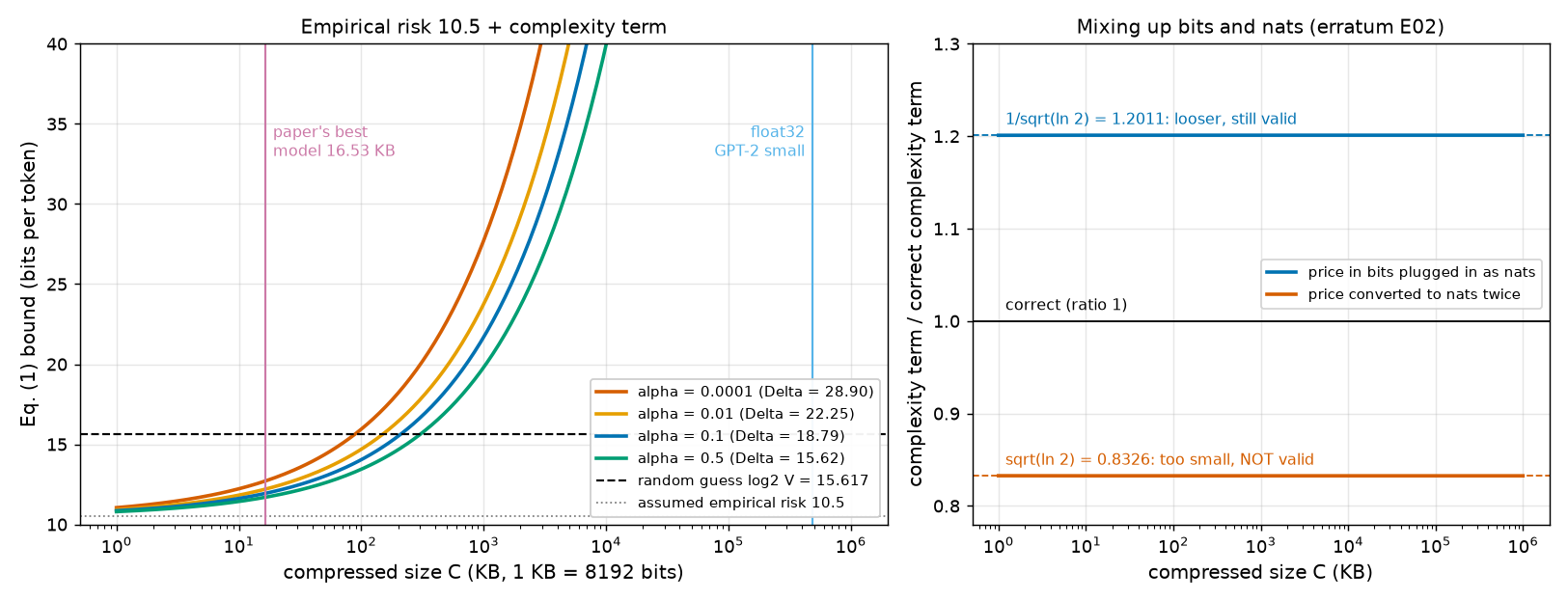
How large may a compressed model be before the bound becomes useless? For the paper's setting the answer is 76.6 to 280.7 KB, against 483,162 KB for GPT-2 small stored in float32.
What happens if bits and nats are mixed up, as the paper's notation invites? (Answer: the bound gets at most 1.2011 times looser in its complexity term, and stays valid.)

Intuition (and where the analogy breaks)¶

Everything in this section is MY EXPLANATION.

Think of the guarantee as a parcel you send to a sceptical recipient. The parcel says "this model works on new text". Before the recipient believes it, you pay postage. The postage depends on how long a message you need to tell the recipient exactly which model you mean.

A model that can be described in a few kilobytes costs little postage. Its guarantee is almost as tight as its training loss.
A model that needs half a gigabyte to describe costs so much postage that the guarantee says nothing.
The postage is paid out of a budget set by the amount of data. More documents, larger budget.

Training finds a model; compression writes down its description; the bound charges for the description's length. A model that is both accurate on the training documents and short to describe gets a strong certificate. This is the paper's whole strategy.

Where it breaks.

Postage grows like a square root, not linearly. Doubling the message length multiplies the complexity term by \(\sqrt 2\), not by 2. Large models are penalized less than linear postage would suggest, but a 29,225-fold difference in size (float32 GPT-2 small versus the paper's 16.53 KB model; script section [2]) still matters enormously.
The recipient already knows a lot, for free. The message only has to be decodable by someone who already holds the architecture, the random seeds, the decompression program and the list of hyperparameter values agreed before training. A real courier charges for every byte; here, everything fixed in advance travels free (Chapter 13, conditioning on the architecture).
The rate card is printed before the parcel exists. The price of every possible message is fixed before the data are seen. You cannot negotiate a discount for the particular model you ended up with (Chapter 11, cheating prior).
The parcel is the compressed model, not the original. What the guarantee covers is exactly the model the recipient can rebuild from the message, not the network you had before compressing it.

Precise definition¶

Everything in this section is MY EXPLANATION unless tagged.

What the paper says¶

PAPER §4.1, p. 4 For a bounded risk and a finite hypothesis space with a prior, the paper states Eq. (1). It then adopts the Solomonoff prior, with the architecture given as input, and writes the chain

\[ \log\frac{1}{P(h)} \le K(h\mid A)\log 2 \le C(h)\log 2 + 2\log C(h), \]

where \(C(h)\) is the number of bits needed to represent \(h\) with a coding scheme specified in advance. It concludes that hypotheses with both low empirical risk and small compressed size give strong bounds even for large models that can represent many hypotheses.

MY EXPLANATION In this explainer's notation (architecture \(\mathcal A\), natural log \(\ln\)), and with the direction of the first step corrected (erratum E01, Chapter 13), the chain reads \(\ln(1/P(h)) \le K(h\mid\mathcal A)\ln 2 \le C(h)\ln 2 + 2\ln C(h)\). The paper's bare "log" must be \(\ln\) here, because the chain feeds Eq. (1), whose logarithms are natural (erratum E02, below).

Compressed size¶

The compressed size \(C(h)\) of a hypothesis is the number of bits in the message that a fixed compressor (Chapter 12) outputs for \(h\). "Fixed" means: chosen before the training data are seen, together with everything the decompressor may use. In the paper that is the architecture, the random seeds that regenerate the starting weights, the decompression program, and the list of hyperparameter values that will be tried.

In the paper, the message holds the trained subspace coordinates after quantization (rounding each number to one of a few shared values, the quantization levels; Chapter 21) and arithmetic coding (Chapter 22). Units: bits. One KB is 8,192 bits (erratum E35).

The compression prior inequality¶

The price of a model of \(C\) bits is

\[ \ln\frac{1}{P(h)} = C(h)\ln 2 + 2\ln C(h) \quad\text{nats}. \]

Read it in two parts:

\(C(h)\ln 2\): the message itself. \(C\) bits are \(C\ln 2\) nats (Chapter 3). Each extra bit halves the prior weight.
\(2\ln C(h)\): the length header. It is \(2\log_2 C\) bits converted to nats. It pays for telling the decoder where the message ends, so that the set of all messages is prefix-free (Chapter 12).

For the paper's best bits-per-token model, \(C = 135{,}434.26\) bits (16.5325 KB, read from Fig. 2 by fig_extract.py). Then \(C\ln 2 = 93{,}875.88\) nats and \(2\ln C = 23.63\) nats. The header is 0.025 % of the price (script section [2]).

Why "\(\le\)" became "\(=\)". The paper derives this as an upper bound on the Solomonoff prior's price, with dropped constants (erratum E12). Chapter 12 showed a cleaner route: define the prior directly from the compressor, \(P(h) = C(h)^{-2}\,2^{-C(h)}\) (the length prior). Its weights add up to at most 0.644934 (ch12_kraft.py), so it is a legal prior, and its price is exactly \(C\ln 2 + 2\ln C\). No incomputable \(K\) and no hidden constant are needed. This chapter uses that route.

Hyperparameter bits¶

PAPER App. C, p. 15 When the authors optimize over hyperparameters such as the LoRA rank \(r\) and the subspace dimension \(d\), they count those choices in the description of \(h\), which becomes \(h = (\theta, d, r)\). A hyperparameter chosen from \(N\) values listed in advance costs \(\log_2 N\) bits. The paper notes that this is the same as paying for a union bound over the choices. PAPER §6.1, p. 7 The bits for \(d\), \(r\), the smoothing weight \(\alpha\), the learning rate and the number of quantization levels are added to the model's size.

MY EXPLANATION Two of these symbols belong to later chapters; in one line each: the subspace dimension \(d\) is the number of trainable coordinates the model is squeezed into (Chapter 18), and the smoothing weight \(\alpha\) sets how much of a uniform guess is mixed into each prediction so that the loss of a token has a ceiling (Chapter 16). The LoRA rank \(r\) is from Chapter 19 and the learning rate from Chapter 7.

Hyperparameter bits are the bits paid to name which point of a grid of \(N\) settings, fixed before training, the model uses: \(\log_2 N\) bits, i.e. \(\ln N\) nats. PAPER App. E, pp. 16–17 The grid is 6 values of \(d\), 2 of \(r\), 3 learning rates, 8 values of \(\alpha\), and 2 numbers of quantization levels. MY EXPLANATION That is \(N = 6\cdot2\cdot3\cdot8\cdot2 = 576\) settings, so the hyperparameter bits are \(\log_2 576 = 9.1699\) bits \(= 6.3561\) nats (script section [3]).

The compression bound¶

Putting the pieces into Eq. (1) gives the compression bound:

The compression bound (Eq. 1 with the compression prior)

Fix before seeing any data: an architecture \(\mathcal A\), random seeds, a compressor and its decompressor, a grid of \(N\) hyperparameter settings, a confidence parameter \(\delta\), the number of documents \(m\), and for every hypothesis an interval of width \(\Delta\) containing its loss on any document. Draw \(m\) training documents i.i.d. Then, with probability at least \(1-\delta\) over this draw, every hypothesis \(h\) that the decompressor can produce from a grid index and a message of \(C(h)\ge 2\) bits satisfies

\[ R(h) \;\le\; \hat R(h) \;+\; \Delta\sqrt{\frac{C(h)\ln 2 + 2\ln C(h) + \ln N + \ln\frac{1}{\delta}}{2m}} . \]

In particular it holds for the trained, compressed hypothesis \(\hat h\), however it was chosen.

Every symbol, with units:

Symbol	Meaning	Units
\(R(h)\)	expected loss of \(h\) on a fresh document	loss units (bits per token, or a fraction for top-k error)
\(\hat R(h)\)	average loss of \(h\) on the \(m\) training documents	loss units
\(\Delta\)	width of the interval containing one document's loss	loss units
\(C(h)\)	length of the compressed message for \(h\)	bits (a count)
\(C(h)\ln 2\)	the message converted to nats	nats
\(2\ln C(h)\)	the length header in nats	nats
\(\ln N\)	hyperparameter bits in nats (\(\log_2 N\) bits \(\times\ln 2\))	nats
\(\ln(1/\delta)\)	price of the confidence level	nats
\(m\)	number of training documents	count

Everything under the square root is in nats divided by a count, so it is a pure number; multiplying by \(\Delta\) gives loss units. The probability is over the random draw of the \(m\) documents. The compressor, grid, \(\delta\), \(m\) and \(\Delta\) are fixed. The trained hypothesis \(\hat h\), and with it \(C(\hat h)\) and \(\hat R(\hat h)\), are random, because they depend on the documents.

MY EXPLANATION Two refinements are needed before the numbers match the paper's tables, and both belong to later chapters. The width \(\Delta\) depends on \(\alpha\), \(\Delta(\alpha) = \log_2(1 + (1-\alpha)V/\alpha)\) bits per token (Chapter 16), with \(V = 50{,}257\) the vocabulary size SOURCE: GPT-2 tokenizer; never printed in the paper, erratum E36. And the paper's Eq. (3), which Chapter 17 derives, is the same bound with \(\hat R(h)\) estimated on \(n = 10{,}000\) randomly chosen documents instead of all \(m\); it adds a second term \(\Delta\sqrt{\ln(1/((1-s)\delta))/(2n)}\) and replaces \(\ln(1/\delta)\) by \(\ln(1/(s\delta))\), with \(s = n/(n+m)\).

The bound applies to the compressed model¶

The certified object is the hypothesis the decoder rebuilds from the message: the quantized model, with its chosen \(\alpha\). It is not the network that existed before quantization.

PAPER App. C, Algorithm 1, p. 15 Algorithm 1 is consistent with this: it quantizes the trained weights first, then computes the training error of the quantized model with prediction smoothing, then its compressed size.

MY EXPLANATION If you measured \(\hat R\) on the unquantized network and \(C\) on the quantized one, the two terms would describe different hypotheses, and Eq. (1) would cover neither combination.

The Note on finite hypothesis spaces¶

PAPER §A.1 Note, p. 13 Theorem A.1 assumes a finite hypothesis space. The paper's Note argues that this holds for real networks: they are programs of finite size, their weights are floating-point numbers with finitely many possible values, and a compressed model is again a finite string of bits. It adds that, despite the name, finite-hypothesis bounds tell us not to count hypotheses but to ask which ones are likely a priori, and that the bounds are often tighter for larger models.

MY EXPLANATION The finite-hypothesis-space Note makes two separate points.

Finiteness is real but irrelevant to the size of the bound. GPT-2 small has \(D = 123{,}689{,}472\) parameters; in float32 (Chapter 10) that is at most \(2^{32D}\) networks, a finite number. Counting them gives a price of 3,958,063,104 bits and a complexity term of 245.86 bits per token at \(\Delta = 18.787\) (script section [2]; Chapter 11 found the same). The count is finite and useless.
The compression prior never looks at the count. The price depends only on \(C(\hat h)\), the length of the one message actually sent. How many other hypotheses exist does not appear anywhere in the bound. In fact the set of all decodable messages has no upper limit on length, so the hypothesis space of the compression prior is endless (countably infinite). Chapter 11 showed that Theorem A.1 holds for such spaces too, as long as the weights add up to at most 1.

The last sentence of the Note ("often tighter for larger models") is a claim about Table 3 and Figure 3; Chapter 26 checks it.

The complexity budget¶

Turn the bound around. Fix a target bound \(T\) (for bits per token, usually the random-guess level \(\log_2 V = 15.617\), below which the bound is non-vacuous) and an empirical risk \(\hat R\). The complexity budget is the largest compressed size \(C\) for which \(\hat R\) plus the complexity term stays at or below \(T\):

\[ C_{\max} = \max\Big\{C \,:\, \hat R + \Delta\sqrt{\tfrac{C\ln 2 + 2\ln C + \ln N + \ln(1/\delta)}{2m}} \le T\Big\}. \]

Because the left side grows with \(C\), the set is an interval and \(C_{\max}\) is found by solving one equation (deeper block "Solving for the budget").

The bits-versus-nats audit¶

A bits-versus-nats audit checks, for each term under the square root, whether it is in nats as Eq. (1) requires. The typical mistake is to plug the compressed size in bits, \(C + 2\log_2 C\), directly into the place of \(\ln(1/P(h))\).

Paper errata E02 and E52: the log base is never stated, and Algorithm 1 mixes bits and nats

PAPER §4.1, p. 4; App. C, Algorithm 1 lines 6 and 20, p. 15 Eq. (1) and the chain write "log" without a base. Algorithm 1 line 20 returns the message size plus "2 × log(message_size)", and line 6 stores that value under the name "log 1/P(h)" before passing it to the bound.

MY EXPLANATION In Eq. (1) "log" must be \(\ln\) (it comes from undoing \(e^{-2mt^2/\Delta^2}\); Chapter 11). Line 20 adds a header to a size counted in bits, so its "log" must be \(\log_2\), and its output is in bits. Line 6 then calls a number of bits "\(\log 1/P(h)\)"; read with the natural log of Eq. (1), that label is off by the factor \(\ln 2\). Taking the pseudo-code literally would put bits where nats belong. The labelling on line 6 is an addendum to E02, logged as erratum E52.

SOURCE: authors' code, per Chapter 12 The public code multiplies the bit count by np.log(2) before it enters the bound, which is the correct conversion.

MY EXPLANATION The worked example (e) shows that the published 12.12 bits per token matches the correct conversion (12.1222), not the literal pseudo-code (12.3871). And it shows that the literal mix-up could only have made the bound looser: bits plugged in as nats inflate the complexity term by at most \(1/\sqrt{\ln 2} = 1.2011\).

Paper erratum E12: the header term is approximate, and constants are dropped

PAPER §4.1, p. 4; App. C, p. 15 The step \(K(h\mid A)\log 2 \le C(h)\log 2 + 2\log C(h)\) and the split \(K(h) \le K(\theta\mid d,r) + K(d) + K(r)\) are written without additive constants.

MY EXPLANATION An Elias gamma header (Chapter 12) costs \(2\lfloor\log_2 C\rfloor + 1\) bits. For the best model that is 35 bits against \(2\log_2 C = 34.09\) bits, a difference of 0.628 nats (script section [2]), against a price of 93,899.5 nats. The step from \(K\) to \(C\) also hides the length of the decoder (Chapter 13). None of this matters if the prior is the length prior of Chapter 12, which gives \(C\ln 2 + 2\ln C\) exactly for every \(C \ge 2\) (erratum E12).

Worked example with real numbers¶

Everything in this section is MY EXPLANATION unless tagged. All numbers are printed by ch14_budget.py.

Inputs used throughout: \(m = 8{,}009{,}762\) documents [SOURCE: nanoGPT prepare.py split; authors' code default num_docs; erratum E32], \(\delta = 0.05\) SOURCE: authors' code; erratum E31, \(n = 10{,}000\) PAPER §6.1, \(V = 50{,}257\) SOURCE: GPT-2 tokenizer; erratum E36, so \(\log_2 V = 15.617\) bits per token, and 1 KB = 8,192 bits (erratum E35). The interval widths \(\Delta(\alpha)\) come from Theorem A.2 (Chapter 16); for example 18.787 bits per token at \(\alpha = 0.1\) and 17.2020 at \(\alpha = 0.25\).

(a) The price of a compressed model, and its complexity term¶

Script section [2] evaluates \(C\ln 2 + 2\ln C\) and the Eq. (1) complexity term \(\Delta\sqrt{(\text{price} + \ln(1/\delta))/(2m)}\) for several sizes (no hyperparameter bits yet).

\(C\) (KB)	\(C\) (bits)	\(2\log_2 C\) (bits)	gamma header (bits)	price (nats)	term, \(\Delta = 1\)	term, \(\Delta = 18.787\)
1	8,192	26.00	27	5,696.3	0.0189	0.3544
5	40,960	30.64	31	28,412.5	0.0421	0.7912
10	81,920	32.64	33	56,805.2	0.0595	1.1188
16.53 (paper's best)	135,434	34.09	35	93,899.5	0.0766	1.4384
20	163,840	34.64	35	113,589.2	0.0842	1.5820
50	409,600	37.29	37	283,938.9	0.1331	2.5012
100	819,200	39.29	39	567,853.4	0.1883	3.5371
1,000	8,192,000	45.93	45	5,678,293.5	0.5954	11.1851
483,162 (float32 GPT-2 small)	3,958,063,104	63.76	63	2,743,520,325.2	13.0867	245.8589

What to notice:

The header is negligible. Even for float32 GPT-2 the header is under 64 bits. The price is essentially \(C\ln 2\).
Square-root growth. Going from 10 KB to 1,000 KB (100 times larger) multiplies the term by about 10: 1.1188 to 11.1851 bits per token at \(\Delta = 18.787\).
Kilobytes are affordable, megabytes are not. At 100 KB the term is 3.5371 bits per token; added to a training loss near 10.5 that is still below 15.617. At 1,000 KB it is 11.1851, which no realistic training loss can survive.
For top-k error (\(\Delta = 1\)) the paper's 16.53 KB model would pay 0.0766 under Eq. (1).

The 20 KB row reproduces Chapter 12's price of 113,589.2 nats.

(b) Hyperparameter bits¶

Script section [3].

The App. E grid has \(N = 576\) settings: \(\log_2 576 = 9.1699\) bits \(= 6.3561\) nats.
That is 0.0068 % of the best model's message.
Coding each hyperparameter separately with a whole number of bits would cost 10 bits; coding the whole grid with one whole-number index would also cost 10 bits. The fractional 9.1699 bits is legal because a prior need not come from whole-number code lengths (weight \(1/N\) for each setting; Chapter 12).
PAPER Fig. 2, p. 5; erratum E40 Fig. 2 plots 8 values of \(d\), while App. E lists 6. If 8 were searched, the grid has 768 settings and costs 9.5850 bits instead. The difference is under half a bit.

The effect on the bound (worked example (c)) appears only in the fifth decimal.

(c) Reproducing the paper's 12.12 bits per token¶

PAPER Table 1, p. 6 The best bits-per-token bound for GPT-2 small is 12.12. It belongs to a SubLoRA model (SubLoRA is the paper's way of training a model inside a small set of trainable coordinates; Chapter 20). [SOURCE: fig_extract.py, reading Fig. 2 (p. 5) from the PDF's vector data; errata page §F] The model behind it has \(d = 50{,}000\), \(\alpha = 0.25\), smoothed empirical risk 10.5945 bits per token and compressed size 16.5325 KB.

MY EXPLANATION Script section [4] puts these into Eq. (3), with \(\Delta(0.25) = 17.2020\):

hyperparameter bits	price (nats)	first term	second term	bound	paper
none	93,899.51	1.31707	0.21057	12.122180	12.12
\(\log_2 576\)	93,905.87	1.31711	0.21057	12.122225	12.12
24 bits	93,916.15	1.31719	0.21057	12.122297	12.12

All three round to 12.12, and the script asserts this. The first term is Eq. (1)'s complexity term with \(\ln(1/(s\delta))\) in place of \(\ln(1/\delta)\); the second is the price of estimating the risk on 10,000 documents (Chapter 17). Their sum, 1.5276 to 1.5278 depending on the row, matches the complexity 1.5278 that fig_extract.py reads off Fig. 1.

The last row uses 24 bits because, according to the note at the end of the errata page, the authors' code charges 8 bits per \(\alpha\) value tried and accumulates this inside a loop SOURCE: authors' code. Even that overpayment changes the bound by about \(10^{-4}\) bits per token.

(d) The complexity budget¶

Here we ask how large a compressed model may be. We assume a smoothed empirical risk of \(\hat R = 10.5\) bits per token. This is an assumption, chosen near the paper's validation 10.53 (Table 2) and the 10.5945 of example (c). Script section [5] solves for the largest \(C\) that keeps the bound at or below \(\log_2 V = 15.617\):

\(\alpha\)	\(\Delta\) (bits/token)	Eq. (1): max price (nats)	Eq. (1): \(C_{\max}\) (KB)	Eq. (3) + 9.17 bits: \(C_{\max}\) (KB)	float32 GPT-2 / \(C_{\max}\)
0.0001	28.905	502,054	88.4	76.6	6,307×
0.001	25.581	640,969	112.9	99.5	4,857×
0.005	23.254	775,715	136.6	121.8	3,966×
0.01	22.246	847,551	149.3	133.8	3,611×
0.05	19.865	1,062,943	187.2	169.8	2,845×
0.1	18.787	1,188,427	209.3	190.9	2,531×
0.25	17.202	1,417,514	249.6	229.5	2,105×
0.5	15.617	1,719,836	302.9	280.7	1,721×

What to notice:

The budget is hundreds of kilobytes. With the full recipe (subsampling and hyperparameter bits) it ranges from 76.6 KB to 280.7 KB. The paper's best model, at 16.53 KB, sits far inside it.
Float32 GPT-2 small is 483,162 KB = 471.84 MiB (1 MiB = 1,024 KB = 8,388,608 bits). It would have to shrink by a factor of 1,721 to 6,307 to fit the budget.
A larger \(\alpha\) buys budget, because it narrows the interval \(\Delta\). This is not free: a larger \(\alpha\) also raises the empirical risk of a good model (Chapter 16). Here \(\hat R\) was held fixed at 10.5, so the table shows only one side of that trade-off.
Top-1 error is far tighter. With \(\Delta = 1\), the paper's best top-1 training error 0.9148 (Fig. 1, read by fig_extract.py) and the random-guess error \(1 - 1/V = 0.99998\), Eq. (1) leaves room for only 20.5 KB.

(e) The bits-versus-nats audit¶

Script section [7] compares the correct complexity term with two mistakes: plugging the price in bits where nats belong ("bits as nats"), and multiplying an already converted price by \(\ln 2\) again ("converted twice").

\(C\) (KB)	\(\Delta\)	correct	bits as nats	ratio	converted twice	ratio
1	18.787	0.3544	0.4256	1.2010	0.2951	0.8327
16.53	17.202	1.3170	1.5819	1.2011	1.0965	0.8326
100	18.787	3.5371	4.2485	1.2011	2.9449	0.8326
1,000	18.787	11.1851	13.4347	1.2011	9.3122	0.8326

Bits as nats is conservative. A number of bits is larger than the same quantity in nats (by the factor \(1/\ln 2\)), so the price is overstated and the bound is looser. The complexity term grows by the factor \(1/\sqrt{\ln 2} = 1.2011\) at most. The bound remains true, only weaker (erratum E02).
Converting twice is not. It understates the price by the factor \(\ln 2\) and shrinks the term by \(\sqrt{\ln 2} = 0.8326\). The resulting number is not covered by Theorem A.1.
The paper's 12.12 used the right conversion. For the best model, Eq. (3) gives 12.1222 correctly, 12.3871 with bits as nats and 11.9017 converted twice. Only the first rounds to the published 12.12.

(f) Reverse-engineering the "Original Model" bound of 70.76¶

PAPER Table 1, p. 6; Table 2, p. 7 For the ordinary GPT-2 small model ("Original Model"), Table 1 reports a bits-per-token bound of 70.76, and Table 2 a validation loss of 4.35 bits per token. The paper does not say how this bound was computed: which code, which \(\alpha\), which empirical risk (errata E33, E53; §6.2 gives only a one-sentence hint, erratum E67).

[MY EXPLANATION, assumption-laden] Script section [6] asks: if the bound came from Eq. (3) with the compression prior, what compressed size would produce exactly 70.76? We assume a smoothed empirical risk of 4, 5 or 6 bits per token (near the validation 4.35) and try every \(\alpha\) in the grid. "Bits per parameter" divides \(C\) by \(D = 123{,}689{,}472\).

\(\alpha\)	largest possible smoothed loss \(\log_2(V/\alpha)\)	\(C\) for \(\hat R = 4\): MiB (bits/param)	\(\hat R = 5\)	\(\hat R = 6\)	bound with raw float32, \(\hat R = 5\)
0.0001	28.905	14.5 (0.99)	14.1 (0.96)	13.7 (0.93)	383.6
0.001	25.583	18.6 (1.26)	18.0 (1.22)	17.5 (1.19)	340.1
0.005	23.261	22.5 (1.53)	21.8 (1.48)	21.2 (1.44)	309.6
0.01	22.261	24.6 (1.67)	23.9 (1.62)	23.2 (1.57)	296.4
0.05	19.939	30.9 (2.09)	30.0 (2.03)	29.1 (1.97)	265.2
0.1	18.939	34.6 (2.34)	33.5 (2.27)	32.5 (2.20)	251.1
0.25	17.617	41.2 (2.80)	40.0 (2.71)	38.8 (2.63)	230.3
0.5	16.617	50.1 (3.39)	48.6 (3.29)	47.1 (3.19)	209.6

Three readings:

70.76 is "more than vacuous". A smoothed model's per-token loss can never exceed \(\log_2(V/\alpha)\), which is at most 28.905 bits for the grid's smallest \(\alpha\) (Chapter 16). A bound of 70.76 is larger than the worst loss the model could possibly have, so it carries no information at all.
It does not come from raw float32. Counting 32 bits per parameter gives bounds of 209.6 to 383.6, far above 70.76.
It fits a code of about 1 to 3.4 bits per parameter, i.e. 13.7 to 50.1 MiB, for example a quantized model. This is only a consistency check: with the method unstated, we cannot tell which reading is right.

Going deeper¶

Everything in this section is MY EXPLANATION unless tagged.

The six blocks below prove the compression bound from the length prior, show that hyperparameter bits are a union bound, make the finite-hypothesis Note precise, solve for the budget, analyse the bits-versus-nats mix-up exactly, and spell out the assumptions behind example (f).

Going deeper: the compression bound, proved from the length prior

The hypothesis list. Fix, before the data, the architecture \(\mathcal A\), the seeds, the decompressor, and a grid \(G\) of \(N\) hyperparameter settings. A description is a pair \((g, s)\): a grid index \(g\in G\) and a bit string \(s\) of length \(\lvert s\rvert \ge 2\) that the decompressor accepts for setting \(g\). Each description decodes to one hypothesis \(h(g, s)\): a quantized model with its smoothing weight. The hypothesis list \(\mathcal H\) is the list of all \(h(g,s)\) (a hypothesis that two descriptions produce is listed twice, which is allowed; Chapter 11, edge cases).

The prior. For a description of length \(c = \lvert s\rvert\), set

\[ P\big(h(g,s)\big) = \frac{1}{N}\cdot\frac{1}{c^2}\cdot 2^{-c} . \]

The weights add up to at most 1. There are at most \(2^c\) bit strings of length \(c\). So

\[ \begin{aligned} \sum_{g\in G}\sum_{s} P\big(h(g,s)\big) &= \sum_{g\in G}\frac1N\sum_{c\ge 2}\#\{s : \lvert s\rvert = c\}\cdot\frac{1}{c^2}\,2^{-c} \\ &\le \sum_{g\in G}\frac1N\sum_{c\ge 2} 2^{c}\cdot\frac{1}{c^2}\,2^{-c} = \sum_{g\in G}\frac1N\sum_{c\ge 2}\frac{1}{c^2} \\ &= \sum_{c\ge2}\frac1{c^2} < 1 . \end{aligned} \]

Line 1 groups strings by length. Line 2 uses the count bound and cancels \(2^c\) against \(2^{-c}\). Line 3 uses that the \(N\) grid points each contribute \(1/N\) times the same sum. The last sum is below 1 by the telescoping argument of Chapter 12: \(1/c^2 < 1/(c-1) - 1/c\) for \(c\ge 2\), so every partial sum is below \(1\). (Its value is \(\pi^2/6 - 1 = 0.644934\).)

No prefix-free property was needed explicitly: the factor \(1/c^2\) plays the role of the length header.

The price. Take \(\ln\) of \(1/P\):

\[ \ln\frac{1}{P(h)} = \ln N + 2\ln c + c\ln 2 , \]

i.e. \((c + 2\log_2 c + \log_2 N)\) bits, converted to nats. With \(c = C(h)\) this is the expression under the square root of the compression bound, minus the \(\ln(1/\delta)\).

The bound. The prior was fixed before the data and its weights add up to at most 1, so Theorem A.1, in the countable form proved in Chapter 11, applies: with probability at least \(1-\delta\) over the \(m\) documents, every listed hypothesis satisfies Eq. (1) with this price. The trained, compressed \(\hat h\) is listed (training produced some grid point \(g\), and the compressor some message \(s\)), so the bound holds for it. \(\square\)

Algorithm 1's order. PAPER App. C, Algorithm 1 lines 19–20, p. 15 The pseudo-code adds the hyperparameter bits to the message size before adding the header, i.e. charges \(C' + 2\log_2 C'\) bits with \(C' = c + \log_2 N\). MY EXPLANATION That is also a legal prior: \(P = 2^{-c}/(N\,(c + \log_2 N)^2)\), and since \((c + \log_2 N)^2 \ge c^2\), every weight is at most the one above, so the sum is again below 1. The two orders differ by \(2\log_2((c+\log_2 N)/c)\) bits, \(1.95\times 10^{-4}\) bits for the best model (script section [3]). The authors' code uses the first order (Chapter 12); pacbound follows the code.

What is random. The documents. Hence \(\hat h\), its grid point, its message, \(C(\hat h)\) and \(\hat R(\hat h)\). What is fixed: everything the decoder knows, the prior, \(\delta\), \(m\), and the width of each hypothesis's interval (for smoothed models, \(\Delta(\alpha)\) with \(\alpha\) read from the grid index; the per-hypothesis width is covered by the edge-case block of Chapter 11).

Going deeper: hyperparameter bits are a union bound over the grid

PAPER App. C, p. 15 The paper says paying \(\log_2 N\) bits is equivalent to paying for a union bound over the choices. MY EXPLANATION Here is the equivalence.

Route 1: separate bounds, then a union. For each grid point \(g\), suppose we have a prior \(P_g\) over the models of that grid point and prove Eq. (1) with failure probability \(\delta/N\). Each such bound fails with probability at most \(\delta/N\), so by the union bound (Chapter 10) all \(N\) hold together with probability at least \(1-\delta\). The price inside the square root is \(\ln(1/P_g(h)) + \ln(N/\delta)\).

Route 2: one prior. Use \(P(h) = P_g(h)/N\) and failure probability \(\delta\). The price is \(\ln(1/P_g(h)) + \ln N + \ln(1/\delta)\).

Since \(\ln(N/\delta) = \ln N + \ln(1/\delta)\), the two routes give identical bounds. Script section [3] checks the numbers: \(\ln(576/0.05) = 9.3518\) nats in both forms.

What must be paid for, and what need not be. The decoder needs \(d\) and \(r\) to interpret the message (the same string of quantized numbers means different models for different \(d\) and \(r\)), and it needs \(\alpha\) to make predictions. Those are part of the description. The learning rate is different: it influences which message training produces, but the decoder does not need it to rebuild the model. Two models trained with different learning rates and the same \(d\), \(r\), \(\alpha\) are two different messages in the same list, and the union bound already covers choosing between them. So the paper's \(\log_2 3 = 1.5850\) bits for the learning rate are an overpayment. It is harmless (conservative) and tiny.

What these bits do not cover. The paper also selects \(\alpha\) and \(d\) by computing the bound on the same 10,000 subsampled documents. The hyperparameter bits pay for the selection in the first term of Eq. (3), but not in its second (subsampling) term, which is a bound for one fixed hypothesis (erratum E07; Chapter 17).

Going deeper: the finite-hypothesis Note, made precise

How many float32 networks are there? A float32 number is a pattern of 32 bits, so a network with \(D\) parameters is one of at most \(2^{32D}\) patterns (Chapter 10). Some patterns are not ordinary numbers (infinities, "not a number" codes) and some represent the same value (\(+0\) and \(-0\)), so the true count of distinct functions is smaller, but finite. For \(D = 123{,}689{,}472\) the uniform-prior price is \(32D\ln 2 = 2.7435\times10^{9}\) nats (Chapter 11), and the resulting complexity term is 245.86 bits per token.

The Note's two claims, separated. (1) Finiteness: true, and enough to apply Theorem A.1 literally with a uniform prior. (2) "Count less, weigh more": the paper's bound uses the compression prior, whose price is \(C\ln 2 + 2\ln C + \ln N\) for the message actually sent. The size of the list does not enter.

Why "finite" is not even needed. The list in the previous block has descriptions of every length, so it is countably infinite. Theorem A.1's proof uses only the union bound and \(\sum_h P(h) \le 1\), both of which hold for countable lists (Chapter 11, edge cases). If one insists on finiteness, cap the message length at, say, \(2^{64}\) bits; the prior and every price stay the same.

The hypothesis is a function, so its evaluation must be fixed too. A hypothesis maps a document to a loss. The decoded weights determine that function only together with the procedure that evaluates the network (arithmetic precision, order of operations, the smoothing formula). That procedure is part of what is fixed in advance. In practice, tiny floating-point differences between machines change a per-token loss in far-off decimals; the bound is about the function as evaluated by the fixed procedure.

Larger architectures are not penalized by their size. The architecture is given to the decoder for free, so a bigger architecture costs nothing by itself. It matters only through \(C(\hat h)\), the message needed to pin down the trained model within it. This is the mechanism behind the Note's last sentence; whether the data support "tighter for larger models" is checked in Chapter 26.

Going deeper: solving for the budget

Step 1: the largest affordable price. Write \(\varepsilon = T - \hat R\) for the slack (loss units) and \(B = \ln(1/P(h))\) (nats). For Eq. (1),

\[ \Delta\sqrt{\frac{B + \ln(1/\delta)}{2m}} \le \varepsilon \iff B \le B_{\max} = \frac{2m\varepsilon^2}{\Delta^2} - \ln\frac1\delta , \]

as in Chapter 11 (divide by \(\Delta\), square both non-negative sides, rearrange). For Eq. (3), first subtract the second term from the slack, \(\varepsilon' = \varepsilon - \Delta\sqrt{\ln(1/((1-s) \delta))/(2n)}\), then use \(\ln(1/(s\delta))\) in place of \(\ln(1/\delta)\).

Step 2: from price to size. Solve \(C\ln 2 + 2\ln C + \ln N = B_{\max}\) for \(C\). The left side is increasing in \(C\) (its derivative \(\ln 2 + 2/C\) is positive), so there is exactly one solution and every smaller \(C\) also fits. The script finds it by bisection (scipy.optimize.brentq) and checks that plugging \(C_{\max}\) back in gives exactly \(T\) (assertions in section [5]).

A hand formula. Ignoring the header, \(C \approx (B_{\max} - \ln N)/\ln 2\). Including it, one fixed-point step \(C \approx (B_{\max} - \ln N - 2\ln C_0)/\ln 2\) with \(C_0\) the first approximation is accurate to a fraction of a bit, because \(2\ln C\) changes very slowly.

Units check. \(\varepsilon\) and \(\Delta\) are both in bits per token, so \(\varepsilon/\Delta\) is a pure number; \(2m(\varepsilon/\Delta)^2\) is then a pure number interpreted as nats, because Eq. (1) is in nats. Dividing nats by \(\ln 2\) gives bits; dividing bits by 8,192 gives KB.

Example. At \(\alpha = 0.1\): \(\varepsilon = 15.617 - 10.5\), \(\Delta = 18.787\), and \(B_{\max} = 1{,}188{,}427\) nats (script section [5]), which is \(C_{\max} = 209.3\) KB under Eq. (1).

Going deeper: bits versus nats, exactly

Let \(b = C + 2\log_2 C + \log_2 N\) be the price in bits and \(\ell = \ln(1/\delta)\). The correct price is \(b\ln 2\) nats. The three versions of the complexity term are

\[ t_{\text{right}} = \Delta\sqrt{\frac{b\ln 2 + \ell}{2m}}, \qquad t_{\text{bits}} = \Delta\sqrt{\frac{b + \ell}{2m}}, \qquad t_{\text{twice}} = \Delta\sqrt{\frac{b(\ln 2)^2 + \ell}{2m}} . \]

Bits as nats is always looser. Since \(\ln 2 < 1\) and \(b > 0\), \(b > b\ln 2\), so \(t_{\text{bits}} > t_{\text{right}}\). The bound with \(t_{\text{bits}}\) is larger than a valid bound, hence also valid. The ratio is

\[ \frac{t_{\text{bits}}}{t_{\text{right}}} = \sqrt{\frac{b + \ell}{b\ln 2 + \ell}} . \]

It increases with \(b\) (the derivative of \((b+\ell)/(b\ln 2+\ell)\) in \(b\) is \(\ell(1-\ln 2)/(b\ln 2+\ell)^2 > 0\)), and as \(b\to\infty\) it tends to \(\sqrt{1/\ln 2} = 1.2011\). For \(b\) near 0 it is close to 1, because then the \(\ell\) term dominates. So the inflation is at most 1.2011, reached for large models (script section [7]: already 1.2010 at 1 KB).

Converting twice is always too small. The same argument with \((\ln 2)^2\) in place of \(\ln 2\) gives a ratio that decreases towards \(\sqrt{\ln 2} = 0.8326\). A margin smaller than Theorem A.1's is not covered by the theorem, so a bound computed that way is not certified (it may still happen to be true, but nothing guarantees it).

The other logarithms. The header term \(2\ln C\) (nats) is \(2\log_2 C\) bits times \(\ln 2\); writing it as \(2\log_2 C\) "nats" is a bits-as-nats slip of a few dozen nats, conservative. \(\ln(1/\delta)\) must be natural; with \(\log_2 20\) in place of \(\ln 20\) it would again be conservative, because \(\log_2 x > \ln x\) for \(x > 1\). The general rule: any quantity in nats replaced by the same quantity in bits makes Eq. (1) looser; the reverse makes it invalid.

Going deeper: the assumptions behind example (f)

What we assumed. (1) The original model's bound was computed with Eq. (3) and the compression prior, \(C\ln 2 + 2\ln C\) nats, with no hyperparameter bits. (2) Its smoothed empirical risk is between 4 and 6 bits per token. Smoothing a model whose unsmoothed validation loss is 4.35 bits per token can raise or lower its loss slightly (Chapter 16 shows how), so the range is a guess. (3) \(\alpha\) is one of the grid's eight values.

What we solved. For each \((\alpha, \hat R)\): \(70.76 = \hat R + t_1(C) + t_2\), with \(t_2\) the subsampling term and \(t_1\) the first term of Eq. (3). This is the budget calculation of the previous block with \(T = 70.76\).

Why the answer moves so much with \(\alpha\). For a large price the first term is about \(\Delta\sqrt{C\ln 2/(2m)}\), so the \(C\) needed for a given term scales like \(1/\Delta(\alpha)^2\). From \(\alpha = 0.0001\) (\(\Delta = 28.905\)) to \(\alpha = 0.5\) (\(\Delta = 15.617\)), \(\Delta\) shrinks and the required size grows accordingly, from 14.1 to 48.6 MiB at \(\hat R = 5\).

Why it matters. The paper's Tables 1 and 2 use the 70.76 to say that the ordinary model's bound is vacuous. That conclusion is right (any bound above 15.617 is vacuous), but the number itself is not comparable with the others: it exceeds the largest loss a smoothed model can have, and its construction is not documented (erratum E53). Chapter 25 returns to it.

Paper erratum E53: how the 'Original Model' bound of 70.76 was computed is not stated

PAPER Table 1, p. 6; Table 2, p. 7 The bits-per-token bound for the uncompressed GPT-2 small model is given as 70.76, with no description of the code, the smoothing weight or the empirical risk used (see also erratum E33).

MY EXPLANATION For every \(\alpha\) in the grid, a smoothed model's loss is at most \(\log_2(V/\alpha) \le 28.905\) bits per token, so 70.76 is above the largest possible loss: "more than vacuous". Raw float32 counting would give 209.6 to 383.6 (at an assumed \(\hat R = 5\)), so the number must come from some compressed code; under our assumptions it corresponds to 0.93 to 3.39 bits per parameter (example (f)). No other number in the paper depends on it.

PAPER §6.2, p. 7 One sentence there says that quantization and arithmetic coding alone, without LoRA or a subspace, give vacuous bounds. MY EXPLANATION That partly states the method (a quantized, entropy-coded full model, consistent with the 1 to 3.4 bits per parameter above), but the number of levels, \(\alpha\), the empirical risk and the bound equation remain unstated (erratum E67; Chapter 25).

Common misconceptions¶

Everything in this section is MY EXPLANATION.

Misconception: The bound gets worse with the number of parameters. — Actually: the parameter count never appears. The architecture is given to the decoder for free; only the compressed size of the trained model, \(C(\hat h)\), enters. A 124-million-parameter architecture with a 16.53 KB message pays 93,899.5 nats.
Misconception: The bound certifies the network that came out of training. — Actually: it certifies the hypothesis the decoder rebuilds from the message: the quantized model with its smoothing weight. The empirical risk must be measured on that same model (Algorithm 1 does so).
Misconception: Searching over hyperparameters ruins the bound, or else is free. — Actually: it costs \(\log_2 N\) bits, here \(\log_2 576 = 9.1699\) bits, which changes the bound in the fifth decimal. It is not free (it must be paid, and the grid must be fixed in advance), and the bits do not cover selection on the subsample (erratum E07).
Misconception: Mixing up bits and nats makes the published bounds wrong. — Actually: using bits where nats belong only loosens the complexity term, by at most a factor 1.2011, so such a bound stays valid. The opposite slip (converting twice) would be invalid, and the paper's 12.12 shows the correct conversion was used.
Misconception: "Finite hypothesis space" means the bound counts all float32 networks. — Actually: counting gives 245.86 bits per token for GPT-2 small, useless. The bound uses a prior that weighs each model by its description length, and the number of hypotheses never enters.

Self-test¶

Q1. A model compresses to 40 KB (1 KB = 8,192 bits) and was chosen from the paper's grid of 576 settings. With \(m = 8{,}009{,}762\) SOURCE: nanoGPT; erratum E32, \(\delta = 0.05\) SOURCE: authors' code; erratum E31, \(\alpha = 0.1\) (\(\Delta = 18.787\) bits per token) and a smoothed empirical risk of 10.8 bits per token, compute the price in nats and the Eq. (1) bound. Is it non-vacuous?

Answer

\(C = 40\times 8192 = 327{,}680\) bits. The price is \((C + 2\log_2 C + \log_2 576)\ln 2 = 227{,}162.2\) nats. The complexity term is \(18.787\sqrt{(227{,}162.2 + 2.9957)/(2\times 8{,}009{,}762)} = 2.2372\) bits per token, so the bound is \(10.8 + 2.2372 = 13.0372\) bits per token (script section [8]). It is below \(\log_2 V = 15.617\), so it is non-vacuous. (Eq. (3) would add the subsampling term of Chapter 17.)

Q2. A colleague trains a model in float32, quantizes and arithmetic-codes it to 20 KB, and reports a bound that uses the 20 KB size together with the training loss of the float32 model, which is lower than that of the quantized model. Is the bound valid? What should they report?

Answer

No. The price \(C\ln 2 + 2\ln C\) belongs to the hypothesis the decoder rebuilds from the 20 KB message, the quantized model. The float32 model is a different hypothesis whose own message would be far longer. Combining the price of one with the training loss of the other is not an instance of Eq. (1) for any hypothesis. They should report the training loss of the quantized (and, for bits per token, smoothed) model, as Algorithm 1 does, and say that the guarantee is about that model.

Q3. A paper reports a bits-per-token bound computed by plugging the compressed size in bits, \(C + 2\log_2 C\), directly into \(\ln(1/P(h))\). Is the bound valid? Roughly how much looser is its complexity term than necessary for a model of hundreds of kilobits? What if instead the authors had multiplied an already converted price by \(\ln 2\) again?

Answer

Valid but loose. Bits overstate a price in nats by the factor \(1/\ln 2\), so the complexity term is multiplied by \(\sqrt{(b + \ell)/(b\ln 2 + \ell)}\), which for a large price \(b\) is essentially \(1/\sqrt{\ln 2} = 1.2011\) (1.2011 already at 16.53 KB; script section [7]). A bound larger than a valid bound is valid. Converting twice shrinks the term by \(\sqrt{\ln 2} = 0.8326\); the result is smaller than Theorem A.1's margin and is not certified. For the paper's best model the three versions give 12.1222 (correct), 12.3871 and 11.9017.

Code for this chapter¶

Run it from the project root:

.venv/Scripts/python explainer/code/ch14_budget.py

Source: ch14_budget.py

"""Chapter 14 demo: compressed size as complexity (the "compression bound").

Claims reproduced / illustrated
  * Paper §4.1, p. 4: ln 1/P(h) <= C(h) ln 2 + 2 ln C(h)  (C(h) in bits; the bare "log" read as ln,
    erratum E02), computed with pacbound.log_inv_prior_nats_from_bits; exact Elias-gamma header
    2 floor(log2 C) + 1 bits for comparison (erratum E12).
  * The complexity term of Eq. (1) for compressed sizes 1 KB ... 1,000 KB (1 KB = 8192 bits, erratum E35),
    for Delta = 1 (top-k error) and Delta(alpha = 0.1) = 18.787 bits/token (Theorem A.2, Ch. 16).
  * App. C, p. 15 / App. E, pp. 16-17: hyperparameter bits, log2 N for a grid of N settings fixed in advance;
    the App. E grid has 6 * 2 * 3 * 8 * 2 = 576 settings -> log2 576 bits.
  * Reproduction of Table 1's 12.12 bits/token from the Fig. 2 model (16.5325 KB, alpha = 0.25, empirical
    10.5945) read by fig_extract.py, via Eq. (3) (Ch. 17) with m = 8,009,762 [SOURCE nanoGPT / authors' code,
    E32], n = 10,000, delta = 0.05 [SOURCE authors' code, E31].
  * Complexity budget [MY ANALYSIS]: largest compressed size for which an assumed empirical risk plus the
    complexity term stays below the random-guess level log2 V (V = 50,257 [SOURCE: GPT-2 tokenizer], E36).
  * Reverse-engineering Table 1's "Original Model" bound 70.76 [MY ANALYSIS, assumption-laden].
  * Bits-vs-nats audit (erratum E02) [MY ANALYSIS]: plugging bits in where nats belong inflates the complexity
    term by at most 1/sqrt(ln 2) = 1.2011 (conservative); converting twice shrinks it (invalid).

Outputs: code/outputs/ch14_budget.txt, docs/assets/fig/ch14_budget.png
"""
from __future__ import annotations

import json
import math
import sys
import time
from pathlib import Path

from scipy.optimize import brentq

import matplotlib
matplotlib.use("Agg")
import matplotlib.pyplot as plt

HERE = Path(__file__).resolve().parent
sys.path.insert(0, str(HERE))
import pacbound as pb  # noqa: E402

OUT_TXT = HERE / "outputs" / "ch14_budget.txt"
FIG = HERE.parent / "docs" / "assets" / "fig" / "ch14_budget.png"
FIG_JSON = HERE / "outputs" / "fig_extract.json"

T0 = time.time()
LINES: list[str] = []


def out(s: str = "") -> None:
    print(s)
    LINES.append(s)


KB = 8192                      # bits per KB (Lotfi et al. 2022 convention; erratum E35)
MIB = 1024 * KB                # bits per MiB = 8,388,608
m, n, delta, V = pb.M_DOCS, pb.N_SUB, pb.DELTA, pb.V_GPT2
LOG2V = pb.random_guess_bpd()
D_GPT2 = pb.gpt2_params(12, 768)          # 123,689,472 (nanoGPT count, Ch. 5)
F32_BITS = 32 * D_GPT2
LN_INV_DELTA = math.log(1 / delta)


def width(alpha: float) -> float:
    return pb.smoothing_interval(alpha)[2]


def c_from_price(price_nats: float, extra_bits: float = 0.0) -> float:
    """Invert pacbound.log_inv_prior_nats_from_bits: the message size C (bits) whose price is price_nats."""
    f = lambda c: pb.log_inv_prior_nats_from_bits(c, extra_bits) - price_nats
    return brentq(f, 2.0, price_nats / pb.LN2 + 100.0, xtol=1e-9)


def eq1_term(c_bits: float, w: float, extra: float = 0.0) -> float:
    return pb.eq1_complexity(pb.log_inv_prior_nats_from_bits(c_bits, extra), m, delta, w)


# ----------------------------------------------------------------------------------------------
fig = json.loads(FIG_JSON.read_text(encoding="utf-8"))
best_pt = min(fig["figure2"]["left"]["bound"], key=lambda p: p["value"])
i_best = fig["figure2"]["left"]["bound"].index(best_pt)
C_KB_BEST = fig["figure2"]["left"]["compressed_size_kb"][i_best]["value"]
RHAT_BEST = fig["figure2"]["left"]["empirical_risk"][i_best]["value"]
C_BEST = C_KB_BEST * KB
top1 = min(fig["figure1"]["left_top1"]["points"]["SubLoRA"], key=lambda p: p["sum"])
GRID = dict(d=len(pb.D_GRID), r=len(pb.R_GRID), lr=len(pb.LR_GRID), alpha=len(pb.ALPHA_GRID),
            Lq=len(pb.QLEVEL_GRID))
N_GRID = math.prod(GRID.values())
H_BITS = math.log2(N_GRID)

out("Chapter 14 - compressed size as complexity  (ch14_budget.py)")
out("[1] Inputs")
out(f"  m = {m:,} docs [SOURCE nanoGPT/authors' code]; n = {n:,}; delta = {delta} [SOURCE authors' code]; "
    f"ln(1/delta) = {LN_INV_DELTA:.4f} nats")
out(f"  V = {V:,} [SOURCE GPT-2 tokenizer]; log2 V = {LOG2V:.3f} bits/token; 1 KB = {KB} bits; "
    f"1 MiB = {MIB:,} bits")
out(f"  Delta(alpha) bits/token: " + ", ".join(f"{a:g}: {width(a):.3f}" for a in pb.ALPHA_GRID))
out(f"  GPT-2 small: D = {D_GPT2:,} params; float32 = {F32_BITS:,} bits = {F32_BITS / KB:,.0f} KB "
    f"= {F32_BITS / MIB:.2f} MiB")

# ----------------------------------------------------------------------------------------------
out("[2] Price of a C-bit model, ln 1/P = C ln2 + 2 ln C (nats), and Eq. (1) complexity term")
out("      C (KB)        C (bits)  2log2C  gamma hdr     price (nats)   Delta=1   Delta=18.787")
rows = [1, 5, 10, C_KB_BEST, 20, 50, 100, 1000, F32_BITS / KB]
for ckb in rows:
    c = ckb * KB
    price = pb.log_inv_prior_nats_from_bits(c)
    out(f"  {ckb:10,.4g} {c:15,.0f} {2 * math.log2(c):7.2f} {pb.elias_gamma_length(int(round(c))):6d}"
        f"   {price:16,.1f}  {pb.eq1_complexity(price, m, delta, 1.0):8.4f}  {pb.eq1_complexity(price, m, delta, width(0.1)):10.4f}")
cb_price = pb.log_inv_prior_nats_from_bits(C_BEST)
out(f"  best model C = {C_KB_BEST:.4f} KB = {C_BEST:,.2f} bits: C ln2 = {C_BEST * pb.LN2:,.2f}, 2 ln C = "
    f"{2 * math.log(C_BEST):.2f} nats; gamma header {2 * math.floor(math.log2(C_BEST)) + 1} bits vs 2log2C = "
    f"{2 * math.log2(C_BEST):.2f} (diff {(2 * math.floor(math.log2(C_BEST)) + 1 - 2 * math.log2(C_BEST)) * pb.LN2:.3f} nats)")
c11 = pb.log_inv_prior_nats_from_bits(16.533 * KB)
out(f"  (rounding to 16.533 KB would give {c11:,.1f} nats; exact read gives {cb_price:,.1f}; diff {c11 - cb_price:.1f});"
    f" header share of price {2 * math.log(C_BEST) / cb_price * 100:.3f} %; float32 / best = {F32_BITS / C_BEST:,.0f}x")

# ----------------------------------------------------------------------------------------------
out("[3] Hyperparameter bits (App. C, App. E grid)")
out("  grid sizes " + ", ".join(f"{k}: {v}" for k, v in GRID.items()) +
    f" -> N = {N_GRID}; log2 N = {H_BITS:.4f} bits = {H_BITS * pb.LN2:.4f} nats")
sep_bits = sum(math.ceil(math.log2(v)) for v in GRID.values())
out(f"  one fixed-length index per hyperparameter: {sep_bits} bits; whole-grid index ceil(log2 N) = "
    f"{math.ceil(H_BITS)} bits; with 8 d values (E40): log2 {N_GRID // 6 * 8} = {math.log2(N_GRID // 6 * 8):.4f} bits")
out(f"  share of the best model's message: {H_BITS / C_BEST * 100:.4f} %;  lr index alone: {math.log2(3):.4f} bits")
u1 = math.log(N_GRID / delta)
u2 = H_BITS * pb.LN2 + LN_INV_DELTA
order_diff = 2 * math.log2((C_BEST + H_BITS) / C_BEST)
out(f"  union over the grid, each point delta/N: ln(N/delta) = {u1:.4f} = ln N + ln(1/delta) = {u2:.4f} nats;"
    f" Alg. 1 header order vs code order: {order_diff:.2e} bits")
assert abs(u1 - u2) < 1e-12

# ----------------------------------------------------------------------------------------------
out("[4] Reproducing Table 1 (12.12) from Fig. 2's best model, Eq. (3), alpha = 0.25")
w25 = width(0.25)
out(f"  C = {C_BEST:,.2f} bits, empirical smoothed risk = {RHAT_BEST:.4f} bits/token, Delta(0.25) = {w25:.4f}")
for extra, lab in [(0.0, "no hyperparameter bits"), (H_BITS, "+ log2 576 bits"), (24.0, "+ 24 bits (code's alpha cost)")]:
    price = pb.log_inv_prior_nats_from_bits(C_BEST, extra)
    t1, t2 = pb.eq3_terms(price, m, n, delta, w25)
    b = RHAT_BEST + t1 + t2
    out(f"  {lab:31s} price {price:,.2f} nats: terms {t1:.5f} + {t2:.5f}; bound {b:.6f} (paper 12.12, diff {b - 12.12:+.4f})")
    assert round(b, 2) == 12.12
eq1_best = eq1_term(C_BEST, w25, H_BITS)
out(f"  Eq. (1) only (all m docs, no subsampling term), with log2 576 bits: complexity {eq1_best:.4f} bits/token")

# ----------------------------------------------------------------------------------------------
RH = 10.5
out(f"[5] Budget: largest C with Rhat + terms <= log2 V = {LOG2V:.3f}; Rhat = {RH} bits/token (ASSUMPTION)")
out("   alpha   Delta   Eq.(1): price nats  C_max KB | Eq.(3)+log2 576 bits: C_max KB   float32/C_max")
budget = {}
for a in pb.ALPHA_GRID:
    w = width(a)
    eps = LOG2V - RH
    p1 = 2 * m * (eps / w) ** 2 - LN_INV_DELTA
    c1 = c_from_price(p1)
    s = n / (n + m)
    t2 = w * math.sqrt(math.log(1 / ((1 - s) * delta)) / (2 * n))
    p3 = 2 * m * ((eps - t2) / w) ** 2 - math.log(1 / (s * delta))
    c3 = c_from_price(p3, H_BITS)
    chk = RH + sum(pb.eq3_terms(pb.log_inv_prior_nats_from_bits(c3, H_BITS), m, n, delta, w))
    assert abs(chk - LOG2V) < 1e-6 and abs(RH + eq1_term(c1, w) - LOG2V) < 1e-6
    budget[a] = (c1, c3)
    out(f"  {a:6g} {w:7.3f} {p1:18,.0f} {c1 / KB:9.1f} | {c3 / KB:28.1f}   {F32_BITS / c3:11,.0f}x")
eps_t = pb.random_guess_topk_error(1) - top1["train_risk"]
p_t = 2 * m * eps_t ** 2 - LN_INV_DELTA
out(f"  top-1 error (Delta = 1): Rhat = {top1['train_risk']:.4f} (Fig. 1 best SubLoRA point), target 1 - 1/V = "
    f"{pb.random_guess_topk_error(1):.5f}: Eq.(1) C_max = {c_from_price(p_t) / KB:.1f} KB")

# ----------------------------------------------------------------------------------------------
TARGET = 70.76
out(f"[6] Reverse-engineering Table 1 'Original Model' {TARGET} (Eq. 3, no hyperparameter bits) [MY ANALYSIS]")
out("   alpha  log2(V/a) | C needed in MiB (bits/param) for Rhat = 4 / 5 / 6 bits/token     | float32 bound, Rhat=5")
for a in pb.ALPHA_GRID:
    w = width(a)
    hi = pb.smoothing_interval(a)[1]
    s = n / (n + m)
    t2 = w * math.sqrt(math.log(1 / ((1 - s) * delta)) / (2 * n))
    cells = []
    for rh in (4.0, 5.0, 6.0):
        price = 2 * m * ((TARGET - rh - t2) / w) ** 2 - math.log(1 / (s * delta))
        c = c_from_price(price)
        cells.append(f"{c / MIB:6.1f} ({c / D_GPT2:4.2f})")
    f32 = 5.0 + sum(pb.eq3_terms(pb.log_inv_prior_nats_from_bits(F32_BITS), m, n, delta, w))
    out(f"  {a:6g} {hi:9.3f} | " + "  ".join(cells) + f"  | {f32:8.1f}")

# ----------------------------------------------------------------------------------------------
out("[7] Bits-vs-nats audit (E02): complexity term with the price in nats (right) vs bits plugged in as nats")
out(f"     C (KB)  Delta  correct   bits-as-nats  ratio | converted twice  ratio   "
    f"(limits 1/sqrt(ln 2) = {1 / math.sqrt(pb.LN2):.4f}, sqrt(ln 2) = {math.sqrt(pb.LN2):.4f})")
for ckb, a in [(1, 0.1), (C_KB_BEST, 0.25), (100, 0.1), (1000, 0.1)]:
    c = ckb * KB
    w = width(a)
    good = pb.eq1_complexity(pb.log_inv_prior_nats_from_bits(c), m, delta, w)
    bad = pb.eq1_complexity(c + 2 * math.log2(c), m, delta, w)
    twice = pb.eq1_complexity(pb.log_inv_prior_nats_from_bits(c) * pb.LN2, m, delta, w)
    out(f"  {ckb:9.4g} {w:6.3f} {good:8.4f} {bad:13.4f} {bad / good:7.4f} | {twice:14.4f} {twice / good:7.4f}")
price_bad = C_BEST + 2 * math.log2(C_BEST) + H_BITS
b_bad = RHAT_BEST + sum(pb.eq3_terms(price_bad, m, n, delta, w25))
price_twice = pb.log_inv_prior_nats_from_bits(C_BEST, H_BITS) * pb.LN2
b_twice = RHAT_BEST + sum(pb.eq3_terms(price_twice, m, n, delta, w25))
b_good = RHAT_BEST + sum(pb.eq3_terms(pb.log_inv_prior_nats_from_bits(C_BEST, H_BITS), m, n, delta, w25))
out(f"  best model, Eq. (3) with log2 576 bits: correct {b_good:.4f} | bits as nats {b_bad:.4f} | converted twice {b_twice:.4f} (paper: 12.12)")

# ----------------------------------------------------------------------------------------------
q_c = 40 * KB
q_price = pb.log_inv_prior_nats_from_bits(q_c, H_BITS)
q_term = pb.eq1_complexity(q_price, m, delta, width(0.1))
out(f"[8] Self-test Q1: C = 40 KB = {q_c:,} bits + log2 576: price {q_price:,.1f} nats; Eq.(1) term (Delta 18.787) "
    f"{q_term:.4f}; bound with Rhat 10.8 = {10.8 + q_term:.4f} bits/token")

# ----------------------------------------------------------------------------------------------
fig_, (ax1, ax2) = plt.subplots(1, 2, figsize=(12.5, 4.8), gridspec_kw={"width_ratios": [1.4, 1]})
xs = [10 ** (k / 40) for k in range(0, 241)]          # 1 KB ... 1e6 KB
cols = {0.0001: "#D55E00", 0.01: "#E69F00", 0.1: "#0072B2", 0.5: "#009E73"}
for a, col in cols.items():
    ys = [RH + eq1_term(x * KB, width(a)) for x in xs]
    ax1.plot(xs, ys, color=col, lw=2, label=f"alpha = {a:g} (Delta = {width(a):.2f})")
ax1.axhline(LOG2V, color="black", ls="--", lw=1.2, label=f"random guess log2 V = {LOG2V:.3f}")
ax1.axhline(RH, color="grey", ls=":", lw=1, label=f"assumed empirical risk {RH}")
ax1.axvline(C_KB_BEST, color="#CC79A7", lw=1.2)
ax1.text(C_KB_BEST * 1.15, 33, f"paper's best\nmodel {C_KB_BEST:.2f} KB", color="#CC79A7", fontsize=9)
ax1.axvline(F32_BITS / KB, color="#56B4E9", lw=1.2)
ax1.text(F32_BITS / KB / 1.15, 33, "float32\nGPT-2 small", color="#56B4E9", fontsize=9, ha="right")
ax1.set_xscale("log")
ax1.set_ylim(10, 40)
ax1.set_xlabel("compressed size C (KB, 1 KB = 8192 bits)", fontsize=11)
ax1.set_ylabel("Eq. (1) bound (bits per token)", fontsize=11)
ax1.set_title("Empirical risk 10.5 + complexity term", fontsize=11)
ax1.legend(fontsize=8.5, loc="lower right", framealpha=0.95)
ax1.grid(alpha=0.3)
ratio = [pb.eq1_complexity(x * KB + 2 * math.log2(x * KB), m, delta, 1.0) /
         pb.eq1_complexity(pb.log_inv_prior_nats_from_bits(x * KB), m, delta, 1.0) for x in xs]
ax2.plot(xs, ratio, color="#0072B2", lw=2, label="price in bits plugged in as nats")
ratio2 = [pb.eq1_complexity(pb.log_inv_prior_nats_from_bits(x * KB) * pb.LN2, m, delta, 1.0) /
          pb.eq1_complexity(pb.log_inv_prior_nats_from_bits(x * KB), m, delta, 1.0) for x in xs]
ax2.plot(xs, ratio2, color="#D55E00", lw=2, label="price converted to nats twice")
ax2.axhline(1 / math.sqrt(pb.LN2), color="#0072B2", ls="--", lw=1)
ax2.axhline(math.sqrt(pb.LN2), color="#D55E00", ls="--", lw=1)
ax2.axhline(1.0, color="black", lw=1)
ax2.text(1.2, 1.0 + 0.012, "correct (ratio 1)", fontsize=9)
ax2.text(1.2, 1 / math.sqrt(pb.LN2) + 0.012, "1/sqrt(ln 2) = 1.2011: looser, still valid", fontsize=9,
         color="#0072B2")
ax2.text(1.2, math.sqrt(pb.LN2) + 0.012, "sqrt(ln 2) = 0.8326: too small, NOT valid", fontsize=9, color="#D55E00")
ax2.set_xscale("log")
ax2.set_ylim(0.78, 1.3)
ax2.set_xlabel("compressed size C (KB)", fontsize=11)
ax2.set_ylabel("complexity term / correct complexity term", fontsize=11)
ax2.set_title("Mixing up bits and nats (erratum E02)", fontsize=11)
ax2.legend(fontsize=8.5, loc="center right")
ax2.grid(alpha=0.3)
fig_.tight_layout()
FIG.parent.mkdir(parents=True, exist_ok=True)
fig_.savefig(FIG, dpi=130)

out("figure: docs/assets/fig/ch14_budget.png")
print(f"runtime {time.time() - T0:.1f} s (console only, so the output file is deterministic)")
OUT_TXT.parent.mkdir(parents=True, exist_ok=True)
OUT_TXT.write_text("\n".join(LINES) + "\n", encoding="utf-8")

Output:

Chapter 14 - compressed size as complexity  (ch14_budget.py)
[1] Inputs
  m = 8,009,762 docs [SOURCE nanoGPT/authors' code]; n = 10,000; delta = 0.05 [SOURCE authors' code]; ln(1/delta) = 2.9957 nats
  V = 50,257 [SOURCE GPT-2 tokenizer]; log2 V = 15.617 bits/token; 1 KB = 8192 bits; 1 MiB = 8,388,608 bits
  Delta(alpha) bits/token: 0.0001: 28.905, 0.001: 25.581, 0.005: 23.254, 0.01: 22.246, 0.05: 19.865, 0.1: 18.787, 0.25: 17.202, 0.5: 15.617
  GPT-2 small: D = 123,689,472 params; float32 = 3,958,063,104 bits = 483,162 KB = 471.84 MiB
[2] Price of a C-bit model, ln 1/P = C ln2 + 2 ln C (nats), and Eq. (1) complexity term
      C (KB)        C (bits)  2log2C  gamma hdr     price (nats)   Delta=1   Delta=18.787
           1           8,192   26.00     27            5,696.3    0.0189      0.3544
           5          40,960   30.64     31           28,412.5    0.0421      0.7912
          10          81,920   32.64     33           56,805.2    0.0595      1.1188
       16.53         135,434   34.09     35           93,899.5    0.0766      1.4384
          20         163,840   34.64     35          113,589.2    0.0842      1.5820
          50         409,600   37.29     37          283,938.9    0.1331      2.5012
         100         819,200   39.29     39          567,853.4    0.1883      3.5371
       1,000       8,192,000   45.93     45        5,678,293.5    0.5954     11.1851
   4.832e+05   3,958,063,104   63.76     63    2,743,520,325.2   13.0867    245.8589
  best model C = 16.5325 KB = 135,434.26 bits: C ln2 = 93,875.88, 2 ln C = 23.63 nats; gamma header 35 bits vs 2log2C = 34.09 (diff 0.628 nats)
  (rounding to 16.533 KB would give 93,902.3 nats; exact read gives 93,899.5; diff 2.8); header share of price 0.025 %; float32 / best = 29,225x
[3] Hyperparameter bits (App. C, App. E grid)
  grid sizes d: 6, r: 2, lr: 3, alpha: 8, Lq: 2 -> N = 576; log2 N = 9.1699 bits = 6.3561 nats
  one fixed-length index per hyperparameter: 10 bits; whole-grid index ceil(log2 N) = 10 bits; with 8 d values (E40): log2 768 = 9.5850 bits
  share of the best model's message: 0.0068 %;  lr index alone: 1.5850 bits
  union over the grid, each point delta/N: ln(N/delta) = 9.3518 = ln N + ln(1/delta) = 9.3518 nats; Alg. 1 header order vs code order: 1.95e-04 bits
[4] Reproducing Table 1 (12.12) from Fig. 2's best model, Eq. (3), alpha = 0.25
  C = 135,434.26 bits, empirical smoothed risk = 10.5945 bits/token, Delta(0.25) = 17.2020
  no hyperparameter bits          price 93,899.51 nats: terms 1.31707 + 0.21057; bound 12.122180 (paper 12.12, diff +0.0022)
  + log2 576 bits                 price 93,905.87 nats: terms 1.31711 + 0.21057; bound 12.122225 (paper 12.12, diff +0.0022)
  + 24 bits (code's alpha cost)   price 93,916.15 nats: terms 1.31719 + 0.21057; bound 12.122297 (paper 12.12, diff +0.0023)
  Eq. (1) only (all m docs, no subsampling term), with log2 576 bits: complexity 1.3171 bits/token
[5] Budget: largest C with Rhat + terms <= log2 V = 15.617; Rhat = 10.5 bits/token (ASSUMPTION)
   alpha   Delta   Eq.(1): price nats  C_max KB | Eq.(3)+log2 576 bits: C_max KB   float32/C_max
  0.0001  28.905            502,054      88.4 |                         76.6         6,307x
   0.001  25.581            640,969     112.9 |                         99.5         4,857x
   0.005  23.254            775,715     136.6 |                        121.8         3,966x
    0.01  22.246            847,551     149.3 |                        133.8         3,611x
    0.05  19.865          1,062,943     187.2 |                        169.8         2,845x
     0.1  18.787          1,188,427     209.3 |                        190.9         2,531x
    0.25  17.202          1,417,514     249.6 |                        229.5         2,105x
     0.5  15.617          1,719,836     302.9 |                        280.7         1,721x
  top-1 error (Delta = 1): Rhat = 0.9148 (Fig. 1 best SubLoRA point), target 1 - 1/V = 0.99998: Eq.(1) C_max = 20.5 KB
[6] Reverse-engineering Table 1 'Original Model' 70.76 (Eq. 3, no hyperparameter bits) [MY ANALYSIS]
   alpha  log2(V/a) | C needed in MiB (bits/param) for Rhat = 4 / 5 / 6 bits/token     | float32 bound, Rhat=5
  0.0001    28.905 |   14.5 (0.99)    14.1 (0.96)    13.7 (0.93)  |    383.6
   0.001    25.583 |   18.6 (1.26)    18.0 (1.22)    17.5 (1.19)  |    340.1
   0.005    23.261 |   22.5 (1.53)    21.8 (1.48)    21.2 (1.44)  |    309.6
    0.01    22.261 |   24.6 (1.67)    23.9 (1.62)    23.2 (1.57)  |    296.4
    0.05    19.939 |   30.9 (2.09)    30.0 (2.03)    29.1 (1.97)  |    265.2
     0.1    18.939 |   34.6 (2.34)    33.5 (2.27)    32.5 (2.20)  |    251.1
    0.25    17.617 |   41.2 (2.80)    40.0 (2.71)    38.8 (2.63)  |    230.3
     0.5    16.617 |   50.1 (3.39)    48.6 (3.29)    47.1 (3.19)  |    209.6
[7] Bits-vs-nats audit (E02): complexity term with the price in nats (right) vs bits plugged in as nats
     C (KB)  Delta  correct   bits-as-nats  ratio | converted twice  ratio   (limits 1/sqrt(ln 2) = 1.2011, sqrt(ln 2) = 0.8326)
          1 18.787   0.3544        0.4256  1.2010 |         0.2951  0.8327
      16.53 17.202   1.3170        1.5819  1.2011 |         1.0965  0.8326
        100 18.787   3.5371        4.2485  1.2011 |         2.9449  0.8326
       1000 18.787  11.1851       13.4347  1.2011 |         9.3122  0.8326
  best model, Eq. (3) with log2 576 bits: correct 12.1222 | bits as nats 12.3871 | converted twice 11.9017 (paper: 12.12)
[8] Self-test Q1: C = 40 KB = 327,680 bits + log2 576: price 227,162.2 nats; Eq.(1) term (Delta 18.787) 2.2372; bound with Rhat 10.8 = 13.0372 bits/token
figure: docs/assets/fig/ch14_budget.png