28. End-to-end mini replication on a CPU¶
Where this fits
Prerequisites: all of Chapters 1–24, especially Chapter 14 (compressed size as complexity), Chapter 15 (documents as the i.i.d. unit), Chapter 16 (prediction smoothing), Chapter 17 (the subsampling bound, Eq. 3), Chapter 20 (SubLoRA), Chapter 21 (quantization), Chapter 22 (arithmetic coding) and Chapter 24 (Algorithm 1). Used later by: Chapter 29. Purpose: run the paper's whole recipe, in miniature, on a laptop, on data whose true distribution we wrote ourselves — and check the certificate against the truth.
The problem this chapter solves¶
Everything in this section is MY EXPLANATION unless tagged.
The paper's headline is a promise. For its best model it says: with probability at least 95 %, the expected bits per token of this (compressed, smoothed) model on new OpenWebText documents is at most 12.12 PAPER §6.2, Table 1, p. 6. (The "95 %" is \(\delta = 0.05\), which the paper never states SOURCE: authors' code; erratum E31.)
Nobody can check that promise directly. The expected risk \(R(h)\) is an average over all documents the web could produce. We only ever see finitely many. A validation set gives an estimate, not the truth, and the authors report validation numbers for a different quantity anyway (erratum E28).
So a reader is asked to trust a long chain: Hoeffding, the prior-weighted union bound, Kraft, smoothing, subsampling, SubLoRA, quantization, arithmetic coding. Each link was proved in Chapters 9–22. But proofs about links do not show the machine running, and a single coding slip anywhere (a forgotten header, a codebook rounded after evaluation, a sum written instead of an average — erratum E03) would silently break the guarantee.
This chapter does what the paper cannot. We write the data-generating process ourselves, as a short program. Then:
- we can draw as many fresh documents as we like, so we can measure the true risk of the certified model to two decimal places;
- we know the exact probability of every document, so we know how good the best possible model is;
- we can run every line of Algorithm 1 and see each number appear.
The question: does the bound really sit above the truth, by how much, and where does the gap come from?
Intuition (and where the analogy breaks)¶
Everything in this section is MY EXPLANATION.
Think of a car maker's crash test. On real roads you cannot stage a crash and measure it precisely. On a test track you build the wall yourself, you know its exact position and hardness, and you can repeat the test as often as you like. If the airbag certificate says "the dummy's head decelerates by at most X", the track lets you check X against a measured value.
Our "test track" is a toy language. Every document is about one of four topics (a farm, the sea, a kitchen, a city), has 2–4 short sentences built from 4 sentence patterns, and uses only that topic's words. A typical document reads "the lazy goat kicks a hen. the dog is old." Because we wrote the rules, we can produce a fresh document whenever we need one, and we can compute exactly how surprising each document is.
The "car" is a tiny GPT-style transformer trained with SubLoRA, quantized and arithmetic-coded exactly as in Algorithm 1. The "certificate" is the paper's Eq. (3). The "measurement" is the model's average loss on 20,000 fresh documents.
Where it breaks.
- A crash test checks one car once. Our check is also a single run: the bound is allowed to fail with probability 5 %, and one run cannot tell a 5 % method from a 0.1 % method. What one run can reveal is a bug that makes the bound fail badly.
- Our toy language is vastly simpler than web text: 29 symbols instead of 50,257 tokens, a few dozen words, 4 sentence patterns, no long-range story. Numbers from the toy do not transfer to GPT-2.
- The "measured" true risk is itself an estimate from finitely many fresh documents. It is very precise here, but it is not exact; we carry its error bar along.
- Passing the check does not prove the bound is valid in general — the theorems do that. The experiment shows the implementation of the theorems behaves as the theorems say.
Precise definition¶
Everything in this section is MY EXPLANATION unless tagged.
The data-generating process¶
A known generator (synthetic data) is a data-generating process written as a program, so that the exact
probability of every document can be computed and unlimited new documents can be drawn. Ours (file ch28_data.py)
draws one document as follows:
- a topic \(t\), uniformly from 4 topics;
- a number of sentences \(k\), uniformly from \(\{2,3,4\}\);
- for each sentence, independently: one of 4 patterns with probabilities 0.3, 0.3, 0.2, 0.2 — "the ADJ NOUN VERB a NOUN.", "a NOUN VERB the ADJ NOUN.", "the NOUN is ADJ.", "the NOUN VERB." — whose slots are filled uniformly from the topic's 8 nouns, 5 verbs and 4 adjectives (two adjectives, "old" and "big", are shared by all topics);
- the sentences are joined by single spaces.
The alphabet has \(V = 29\) symbols: an end-of-text symbol EOT (printed as |), the space, the full stop and the 26
lower-case letters. Documents are drawn independently, so they are i.i.d. by construction. Inside a document the
characters are strongly dependent: spelling, grammar and topic all tie them together.
Three separate random-number streams (seeds) give the \(m\) training documents, the subsample indices and the fresh documents, so none of them can leak into another.
Fresh documents are new independent draws from the generator, used neither for training nor for computing the bound; they play the role of the population.
The pieces of Algorithm 1, in miniature¶
| Item | Paper | This chapter |
|---|---|---|
| alphabet / vocabulary \(V\) | 50,257 GPT-2 tokens PAPER App. E | 29 characters |
| training documents \(m\) | 8,009,762 [SOURCE: nanoGPT prepare.py; authors' code] |
100,000 |
| document length | up to thousands of tokens | at most 118 characters (mean 68.0) |
| subsample \(n\) | 10,000 PAPER §6.1 | 2,000, drawn with replacement |
| architecture | 12 layers, width 768, 12 heads, context 1,024 PAPER App. E | 4 layers, width 64, 4 heads, context 128 |
| parameters \(D\) | 124M | 211,968 |
| LoRA | rank \(r\in\{1,4\}\), \(\alpha_{\text{LoRA}}=32\), on q, v and head PAPER App. E | \(r=4\), \(\alpha_{\text{LoRA}}=32\), on q, v and head: 4,468 LoRA parameters |
| subspace dimension \(d\) | 5,000 – 200,000 PAPER App. E | 256, 576, 1,024, 2,304 |
| quantization levels \(L_q\) | 11, 17 PAPER App. E | 11, 17 |
| smoothing \(\alpha\) | 8 values from 0.0001 to 0.5 PAPER App. E | the same 8 values |
| confidence | \(\delta = 0.05\) SOURCE: authors' code | \(\delta = 0.05\) |
| true risk | unknown | measured on 20,000 fresh documents |
Every document fits in the context window (118 characters plus two EOT symbols is less than 128), so the long-document rule of the paper's Eq. (9) — and its problem, erratum E15 — never arises here.
What is certified¶
A hypothesis is \(h = (\hat w, d, L_q, \alpha)\): the quantized subspace coordinates \(\hat w\) together with the hyperparameters. The random initialization \(\theta_0\), the fixed LoRA initialization \(\phi_0\) and the projector \(P\) are generated from seeds chosen before any data are drawn, so they belong to the architecture \(\mathcal A\) that the decoder gets for free.
The certified model is the exact object the bound is about: the network \(\theta_0 + \mathrm{LoRA}(\phi_0 + P\hat w)\), with the codebook rounded to 16-bit floats, smoothed with the chosen \(\alpha\) (Eq. 2). It is not the unsmoothed network, and not the network before quantization.
Its per-document loss is the bits per character (BPD) of the smoothed model on that document. The document is fed
as [EOT] + characters, and the model must predict the characters and the closing EOT (so a document of 68
characters contributes 69 predictions). Starting from the preceding EOT copies the authors' code
[SOURCE: authors' code, sample_single_document]. The top-1 error of a document is the fraction of those
predictions whose most likely symbol is wrong (erratum E14: the paper's displayed formula counts correct
predictions).
The checks¶
For each certified hypothesis we report
- \(\hat{\hat R}(h)\): the average loss over the \(n = 2{,}000\) subsampled training documents (what the bound uses);
- \(\hat R(h)\): the average over all \(m = 100{,}000\) training documents (affordable at this scale);
- the bound of Eq. (3), computed with
pacbound.eq3_bound; - the bound with the selection fix of erratum E07;
- a true-risk estimate: the average loss on fresh documents, used as a stand-in for \(R(h)\), with a confidence half-width — the \(\pm\) margin around it;
- the random-guess baselines \(\log_2 V\) and \(1 - 1/V\).
The test is: bound \(\ge\) true-risk estimate, for every hypothesis we report.
Worked example with real numbers¶
Everything in this section is MY EXPLANATION unless tagged. All numbers are printed by ch28_mini_sublora.py
(full run, output at the end of the chapter).
Step 0 — the world we built¶
The generator produced \(m = 100{,}000\) training documents of mean length 68.0 characters (longest 118), and a separate set of 20,000 fresh documents.
Because we know the generator, we can score each fresh document with its exact probability \(\Pr[X = x]\) and form \(-\log_2 \Pr[X=x]\) divided by the number of predicted symbols. Averaged over fresh documents this generator's BPD is 0.503 bits per character. A model that knew the rules perfectly would score about this. (It is not quite a hard floor for a per-document average: by favouring short documents a model could undercut it, but by at most 0.0013 bits per character — see the deeper block below.)
For scale: guessing uniformly among 29 symbols costs \(\log_2 29 = 4.858\) bits per character and has top-1 error \(1 - 1/29 = 0.966\).
Step 1 — sanity checks before training¶
- The projector. \(P = (Q_1\otimes Q_2)[\,{:}D,:]\) with \(Q_1, Q_2\) having orthonormal columns from QR factorizations of Gaussian matrices (§5 construction; erratum E08). We pad the LoRA dimension \(D = 4{,}468\) up to \(s^2 = 67^2 = 4{,}489\) and keep the first \(D\) rows (erratum E09: the paper does not say how to handle non-squares). We never build \(P\): \(Pw\) is computed by the reshape trick of the deeper block below. On a small case the trick agrees with the explicit Kronecker product to \(6.0\times10^{-8}\) (rounding error). Dropping 21 rows makes \(P^\top P\) differ from the identity by at most 0.018 for \(d = 1{,}024\) — harmless, because the bound never needs \(P\) to be orthonormal.
- Erratum E10. With the LoRA factors initialized at zero, the gradient of the training loss with respect to \(w\) at \(w = 0\) has norm exactly 0.0 — training could never start. With the standard LoRA initialization (\(A\) random, \(B = 0\)) it is 0.597. So the formula \(\theta_0 + \mathrm{LoRA}(Pw)\) must be read as \(\theta_0 + \mathrm{LoRA}(\phi_0 + Pw)\), as the authors' code does.
Step 2 — the original model (all parameters trained)¶
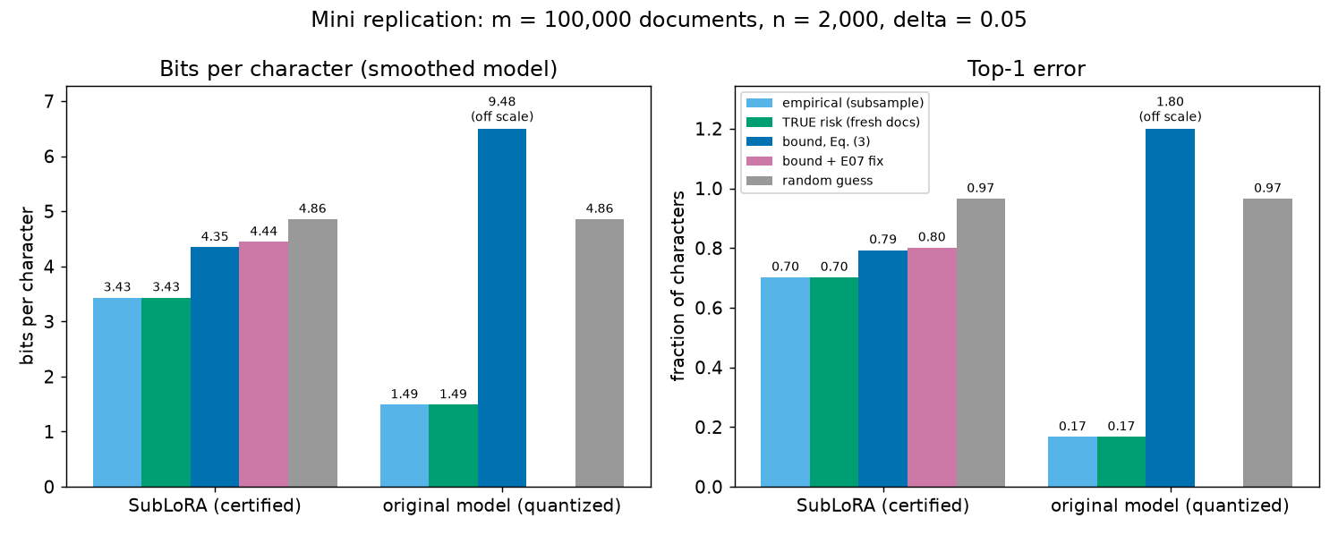
We first train all 211,968 parameters (1,000 Adam steps). On fresh documents the unquantized model scores 0.568 bits per character and top-1 error 0.166 — close to the generator's 0.503. It writes nearly grammatical, on-topic text (samples at the end of the output).
To certify it we must describe it. We quantize all \(D\) numbers to 17 levels (k-means start, 100 steps of quantization-aware training) and arithmetic-code them: 739,961 bits, so \(\ln 1/P(h) = 512{,}929\) nats. That complexity term overwhelms everything. The best bound (at \(\alpha = 0.5\)) is 9.48 bits per character, while the same smoothed model's true risk is 1.488. The bound is vacuous: it is above the 4.858 of random guessing. The top-1 bound is 1.80, above 1, which says nothing at all.
PAPER §6.2, Table 1–2, p. 6–7 This mirrors the paper's "Original Model" column: 70.76 bits per token against a random-guess 15.62, for a model whose validation BPD (4.35) is excellent.
Step 3 — TRAIN_SUBLORA¶
Now the trained object is only \(w\in\mathbb R^d\). All 211,968 base parameters stay at their random initialization \(\theta_0\); the 4,468 LoRA numbers are \(\phi_0 + Pw\). For each \(d \in \{256, 576, 1024, 2304\}\) we train \(w\) for 600 Adam steps.
Step 4 — TRAIN_QUANTIZE¶
For each trained \(w\) and each \(L_q \in \{11, 17\}\): k-means gives an initial codebook \(c\); 150 steps of quantization-aware training then update \(w\) and \(c\) together, with the straight-through estimator (Algorithm 1 line 12 does not say how to differentiate through rounding — erratum E17). Finally the codebook is rounded to 16-bit floats and every entry is snapped to its nearest level. That rounded vector is the one we evaluate — rounding the codebook after evaluation would certify a model different from the one we scored.
Step 5 — GET_COMPRESSED_SIZE¶
Take the best hypothesis of the grid: \(d = 1{,}024\), \(L_q = 11\). We run a real arithmetic coder with exact integer arithmetic, decode the bit string, and check that it returns the 1,024 level indices exactly.
- payload: 3,415 bits — equal to the theoretical limit \(\lceil d\,H(\hat p)\rceil + 1\) = 3,415, where \(H(\hat p)\) is the entropy of the level frequencies;
- header: 297 bits — 11 codebook values at 16 bits plus 11 counts (erratum E18: the paper does not say whether this is counted; we count it, and use \(\lceil\log_2(d+1)\rceil\) bits per count — see the warning below);
- hyperparameters: 6 bits — a uniform choice among \(4\times2\times8 = 64\) values of \((d, L_q, \alpha)\).
Algorithm 1 line 20 adds \(2\log_2\) of the total (base 2, because the message size is in bits — erratum E02), and multiplying by \(\ln 2\) converts to nats: \(\ln 1/P(h) = 2{,}593.6\) nats. The whole model fits in under half a kilobyte.
Step 6 — smoothing and the subsampling bound¶
On the \(n = 2{,}000\) subsampled training documents the smoothed model with \(\alpha = 0.25\) has \(\hat{\hat R} = 3.433\) bits per character. At \(\alpha = 0.25\) the loss interval has width \(\Delta = 6.459\) bits (Theorem A.2). Eq. (3) adds two terms:
Each \(\alpha\) gives a different bound; \(\alpha = 0.25\) was the best of the eight.
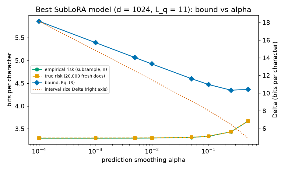
The figure is our analogue of the paper's Fig. 2 (right). Small \(\alpha\) leaves the empirical risk almost unchanged but makes \(\Delta\) huge (right axis of the figure), and \(\Delta\) multiplies both penalty terms. Large \(\alpha\) shrinks \(\Delta\) but pushes the empirical risk up, because every confident prediction loses probability to the uniform mixture. The sweet spot is in between.
4.347 < 4.858: the bound is non-vacuous. With the selection fix of erratum E07 — paying for the 64 candidates that were compared on the same subsample — it is 4.443, still non-vacuous.
Step 7 — the check against the truth¶
On 20,000 fresh documents the same certified model has average loss 3.435 bits per character. Two error bars:
- Hoeffding (valid for any loss in an interval of width \(\Delta\)): \(\pm 0.062\);
- the central limit theorem (CLT) — the fact that an average of many i.i.d. values is approximately normally distributed with standard deviation \(\sigma/\sqrt N\): \(\pm 0.002\).
So the truth is \(3.435 \pm 0.062\) at worst, and the bound 4.347 sits above it. Even after adding the conservative Hoeffding error bar the bound clears the truth by 0.851 bits per character.
The script asserts "bound \(\ge\) true-risk estimate" for every hypothesis it reports: all 8 grid rows for both metrics, plus the four headline numbers. All 20 checks passed.
Step 8 — the gap, and the price of the guarantee¶
Notice three numbers that agree almost perfectly:
| bits per character | |
|---|---|
| \(\hat{\hat R}\) on 2,000 subsampled training documents | 3.433 |
| \(\hat R\) on all 100,000 training documents | 3.435 |
| true risk on 20,000 fresh documents | 3.435 |
This SubLoRA model does not overfit at all — it has only a few thousand bits of freedom, far too few to memorize 100,000 documents. Its real generalization gap is essentially zero. Yet the bound sits about 0.9 bits higher: that difference is almost exactly the two penalty terms (0.737 + 0.177).
We call the gap between a bound and the true risk of the same hypothesis the price of the guarantee. Here it is not caused by overfitting; it is what one pays for a statement that must hold, with probability 95 %, before seeing any fresh data, for whichever of the \(2^{\text{thousands}}\) describable models training happened to pick.
Step 9 — top-1 error¶
The best top-1 hypothesis is \(d = 256\), \(L_q = 11\) (smoothing does not change which symbol is most likely, so \(\alpha\) plays no role and the hyperparameter grid has \(4\times2 = 8\) entries). Its subsample error is 0.702; the two penalty terms are only 0.064 and 0.027 because \(\Delta = 1\) for an error rate. The bound is 0.793 (0.802 with the E07 fix), against random guessing at 0.966 and a true error of 0.702 ± 0.010.
Step 10 — the compression trade-off over d¶
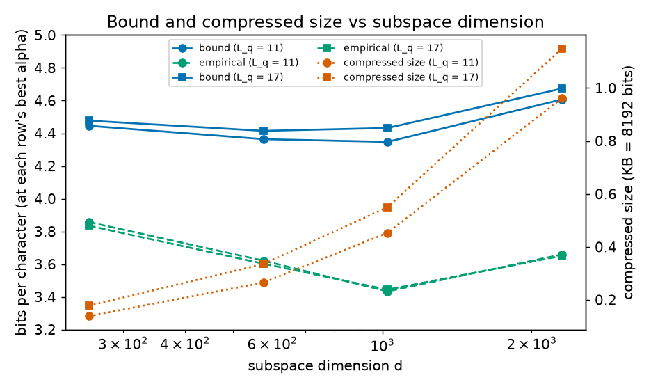
Our analogue of the paper's Fig. 2 (left). The compressed size grows roughly in proportion to \(d\) (from 1,133 to 7,878 bits for \(L_q = 11\)). The empirical risk first falls with \(d\) (more freedom fits the data better) and the bound is best at an intermediate \(d = 1{,}024\). At \(d = 2{,}304\) the larger size pushes the best \(\alpha\) up to 0.5, which in turn raises the smoothed empirical risk — the jump in the dashed curve. Fewer levels (\(L_q = 11\)) give the better bound at every \(d\) in our grid.
Step 11 — what the certified model can do¶
The output ends with 300 characters sampled at temperature 0.8 from both models (the paper's Tables 6–7 do the same PAPER App. F, p. 17–19). The original model writes "a horse finds the big cow. the old dog finds a sheep." The certified SubLoRA model writes letter salad with occasional real words. Its true risk, 3.435 bits per character, is far from the 0.568 of the uncertified original. PAPER Table 2, p. 7; Table 7, p. 19 The paper shows the same pattern: validation BPD 10.53 for SubLoRA against 4.35 for the original, and SubLoRA samples that are gibberish.
Paper erratum E10: the LoRA factors need a fixed nonzero initialization
PAPER §5, Eq. 4, p. 6 writes \(\theta = \theta_0 + \mathrm{LoRA}(Pw)\). Read literally, both LoRA factors are zero at \(w = 0\), and our Step 1 measured the resulting gradient norm: exactly 0.0. The corrected form, used here and in the authors' code, is \(\theta = \theta_0 + \mathrm{LoRA}(\phi_0 + Pw)\) with \(\phi_0\) = (\(A\) random, \(B = 0\)), which gave gradient norm 0.597.
Paper erratum E07: choosing α and d on the same subsample
PAPER §6.1, p. 7 picks the \(\alpha\) and the \(d\) that give the best bound on the \(n\) subsampled documents. The n-term of Eq. (3) covers one fixed hypothesis only. With the union over our 64 compared candidates the n-term grows from 0.177 to the value implied by the "E07" column; the bound goes from 4.347 to 4.443. The conclusion (non-vacuous) survives, as the existing analysis of erratum E07 predicts.
Paper erratum E18 addendum: the width of the count header (listed with the E18 notes in the errata page)
Erratum E18 notes that the paper does not say whether the codebook and the symbol counts are part of the message size; Lotfi et al. (2022) and the authors' code charge \(L_q\lceil\log_2 d\rceil\) bits for the counts. A count can equal \(d\) (if one level were used by every entry), and when \(d\) is a power of two — like our \(d = 256\) and \(d = 1{,}024\) — \(\lceil\log_2 d\rceil\) bits cannot represent the number \(d\). Using \(\lceil\log_2(d+1)\rceil\) bits always works; it costs at most \(L_q\) extra bits (≤ 17), which changes a bound only in the fifth decimal. We use the safe width.
[SOURCE: authors' code, config_sublora_bounds.yaml] A side note, not an erratum: the public default bound
configuration turns quantization-aware training off (max_quant_iters: 0) and uses a uniform grid rather than
k-means (use_kmeans: False), whereas Algorithm 1 and App. C describe k-means plus quantization-aware training. We
follow the paper's description.
Going deeper¶
The blocks below are MY EXPLANATION unless tagged.
Going deeper: the exact probability of a document, and why the generator's BPD is (almost) a floor
The probability. Fix a document string \(x\). Split it at ". " into sentences and each sentence into words. Given a topic \(t\), a sentence string can come from at most one pattern: the word categories (adjectives, nouns, verbs) are disjoint, and the fixed words "the", "a", "is" belong to no category, so the sequence of categories identifies the pattern. If pattern \(j\) (probability \(\pi_j\)) matches and every slot word is in topic \(t\)'s list,
otherwise it is 0. Sentences are independent given \(t\), the number of sentences \(k\) is uniform on \(\{2,3,4\}\), and the topic is uniform on 4 values, so
The string also determines \(k\), so no other combination of choices produces \(x\). The probability is over one draw from the generator; \(x\) is fixed.
Chain rule. A character model assigns \(q(x) = \prod_{i=1}^{L} q(x_i \mid x_{<i})\) to the \(L\) predicted symbols (characters plus the closing EOT). If \(q\) equals the generator's own conditional probabilities, the per-document loss \(-\frac1L\sum_i \log_2 q(x_i\mid x_{<i})\) equals \(-\log_2\Pr[X=x]/L\). Averaging this over fresh documents gives the generator's BPD, 0.503.
Why it is not quite a floor. The risk is a per-document average: each document gets weight 1, so each of its \(L\) symbols gets weight \(1/L\). Write \(p(x)=\Pr[X=x]\) and \(Z = \mathbb E_p[1/L(X)]\), and define the re-weighted distribution \(\tilde p(x) = p(x)/(L(x) Z)\), which sums to 1. For any model \(q\) over documents,
By Gibbs' inequality (Chapter 22) the last sum is smallest when \(q = \tilde p\), not when \(q = p\). The improvement available over the generator is
using \(\tilde p/p = 1/(LZ)\). We estimate this expectation on the fresh documents: 0.0013 bits per character. So no model can beat 0.503 by more than about that (up to the sampling error of the estimate). The same weighting issue is why the paper's per-document bound and a per-token validation BPD are not the same quantity (erratum E28).
Going deeper: the vec trick for P w, and what truncating rows does
Let \(Q_1, Q_2 \in \mathbb R^{s\times t}\) and \(K = Q_1\otimes Q_2 \in \mathbb R^{s^2\times t^2}\). Index the rows of \(K\) by pairs \((a,b)\) and its columns by pairs \((i,j)\), in row-major order, so that by definition of the Kronecker product \(K_{(a,b),(i,j)} = (Q_1)_{ai}(Q_2)_{bj}\). Reshape \(w\in\mathbb R^{t^2}\) row-major into a \(t\times t\) matrix \(W\) with \(W_{ij} = w_{(i,j)}\). Then
So \(Kw\) is the row-major flattening of \(Q_1WQ_2^\top\). This costs about \(2st^2\) multiplications instead of
\(s^2t^2\), and needs no \(s^2\times t^2\) matrix in memory. The script asserts agreement with torch.kron on a small
case.
Orthonormality. By the mixed-product property (Chapter 8), \(K^\top K = (Q_1^\top Q_1)\otimes(Q_2^\top Q_2) = I_t\otimes I_t = I_{t^2}\). Our \(P\) keeps the first \(D\) rows of \(K\). Writing \(R\) for the \(s^2 - D\) dropped rows, \(K^\top K = P^\top P + R^\top R\), hence \(P^\top P = I - R^\top R\). With 21 dropped rows out of 4,489 the deviation is small (0.018 measured). Nothing in the bound needs \(P^\top P = I\): \(P\) is fixed by a seed before the data are drawn, so any \(P\) gives a valid hypothesis class; orthonormality only helps optimization.
Going deeper: why the gradient vanishes when the LoRA factors start at zero (erratum E10)
For one adapted matrix the update is \(\Delta W = c\,BA\) with \(c = \alpha_{\text{LoRA}}/r = 8\). Let \(G = \partial \mathcal L/\partial(\Delta W)\) be the gradient of the training loss with respect to the update. The chain rule gives
The flat LoRA vector is \(\phi = \phi_0 + Pw\), so \(\partial\mathcal L/\partial w = P^\top\,\partial\mathcal L/\partial\phi\). If \(\phi_0 = 0\) then at \(w = 0\) both \(A = 0\) and \(B = 0\), so both partial derivatives above are zero matrices, so \(\partial\mathcal L/\partial\phi = 0\) and \(\partial\mathcal L/\partial w = P^\top 0 = 0\) — for every matrix, every batch. Gradient descent never moves. With \(\phi_0\) = (\(A_0\) random, \(B_0 = 0\)), \(\partial\mathcal L/\partial B = cGA_0^\top\) is nonzero whenever \(G \ne 0\), and training starts. Our measured norms: 0.0 and 0.597.
Going deeper: the exact arithmetic coder and its length guarantee
Let the quantized vector have \(K = d\) symbols, level \(\ell\) occurring \(n_\ell\) times, \(N = \sum_\ell n_\ell = d\), and empirical probabilities \(\hat p_\ell = n_\ell/N\). Arithmetic coding maps the whole sequence to a sub-interval of \([0,1)\) whose width is the product of the probabilities of the symbols:
We do this with Python integers: after \(k\) symbols the interval is \([\mathrm{LOW}, \mathrm{LOW}+\mathrm{WIDTH})/N^k\) with \(\mathrm{WIDTH} = \prod n_{s}\), so nothing is ever rounded.
Length. Choose \(j = \lceil\log_2(1/W)\rceil + 1\) bits (we write \(j\) here because \(\ell\) already indexes the levels). Then \(2^{-j} \le W/2\). Let \(b = \lceil \mathrm{low}\cdot 2^j\rceil\), where \(\mathrm{low}\) is the left end of the final interval. Then \(b/2^j \ge \mathrm{low}\), \(b/2^j < \mathrm{low} + 2^{-j}\) and \((b+1)/2^j < \mathrm{low} + 2\cdot2^{-j} \le \mathrm{low} + W\), so the whole binary interval \([b, b+1)/2^j\) (Chapter 22) lies inside the code interval. Sending the \(j\) bits of \(b\) therefore identifies the sequence, and the code length is at most \(\lceil K H(\hat p)\rceil + 1\). The script searches for the shortest such \(\ell\) and found exactly that limit: 3,415 bits for the best model.
Decodability. The decoder must know \(K\), the levels and the counts. \(K = d\) and \(L_q\) are part of the hyperparameter index (6 bits). The codebook (16-bit floats) and the counts (\(\lceil\log_2(d+1)\rceil\) bits each) form the 297-bit header. The script decodes the payload and asserts it recovers every symbol.
Prefix-freeness. The messages of different hypotheses have different lengths. Algorithm 1 line 20 adds \(2\log_2 C\) bits so that the set of all messages can be made prefix-free (an Elias-type length prefix; Chapter 12), which is what the Kraft inequality needs to turn code lengths into a prior. Strictly, the Elias-gamma prefix costs \(2\lfloor\log_2 C\rfloor + 1\) bits, which can exceed \(2\log_2 C\) by up to one bit (erratum E12); that changes the bound in the fifth decimal. Here \(C = 3{,}415 + 297 + 6\) bits.
For the original model (\(D = 211{,}968\) symbols) the exact big-integer coder would be too slow, so the script charges the proven upper limit \(\lceil D H(\hat p)\rceil + 2\) bits instead of running it.
Going deeper: the bound computation with units, and what is random
Inputs. \(m = 100{,}000\) documents; \(n = 2{,}000\); \(s = n/(n+m)\); \(\delta = 0.05\) SOURCE: authors' code; \(\ln 1/P(h) = 2{,}593.6\) nats; \(\alpha = 0.25\), so by Theorem A.2 (Chapter 16) each smoothed per-character loss lies in \([\log_2(V/\alpha) - \Delta, \log_2(V/\alpha)]\) with \(\Delta = \log_2(1 + (1-\alpha)V/\alpha) = 6.459\) bits per character. A per-document BPD is an average of such numbers, so it lies in the same interval. The script asserts this for every document it scores.
Eq. (3) with the average (erratum E03).
Units: \(\ln 1/P(h)\) and \(\ln 1/(s\delta)\) are in nats (natural logs, as Hoeffding's \(e^{-2mt^2/\Delta^2}\) requires — erratum E02); the ratio under each root is a pure number; multiplying by \(\Delta\) (bits per character) gives bits per character. The printed terms are 0.737 and 0.177.
What is random. The probability "at least \(1-\delta\)" is over two things: the draw of the \(m\) training documents from the generator, and the draw of the \(n\) subsample indices \(\sigma(i)\) (uniformly, with replacement, as in §4.4 — erratum E05). Fixed before any of that: the architecture, \(\theta_0\), \(\phi_0\), \(P\), the grids, the coding scheme (hence the prior). Training is a function of the training documents, so \(\hat h\) is random; the first term survives this because the prior-weighted union bound covers every \(h\) at once (Chapter 11). The second term is a Hoeffding bound for one fixed \(h\) given the training set; it does not cover choosing among 64 candidates on the same subsample. Replacing \(\ln\frac{1}{(1-s)\delta}\) by \(\ln\frac{64}{(1-s)\delta}\) repairs this (erratum E07) and gives 4.443.
The check is itself statistical. The fresh-document average is an estimate of \(R(h)\). The documents are i.i.d. and each loss lies in an interval of width \(\Delta\), so by two-sided Hoeffding, with probability at least 95 % over the fresh draw, \(R(h)\) is within \(\Delta\sqrt{\ln(2/0.05)/(2N)} = 0.062\) of the estimate (\(N = 20{,}000\)). The CLT half-width \(1.96\,\hat\sigma/\sqrt N = 0.002\) is much smaller because the actual spread of per-document losses is far smaller than \(\Delta\); it is approximate (it relies on the normal approximation), which is why we also show Hoeffding. Even "estimate + Hoeffding half-width" stays 0.851 below the bound.
Going deeper: what this experiment shows and what it does not
Shows.
- The whole pipeline — SubLoRA, quantization-aware training, an actually decodable arithmetic code, line 20, smoothing, Eq. (3) — can be implemented so that the bound lands above the measured truth, for every hypothesis we reported (20 checks).
- The qualitative pattern of the paper's Tables 1, 2, 6 and 7 appears at toy scale: a non-vacuous SubLoRA bound, a vacuous bound for the fully trained model, and a certified model much worse than the uncertified one.
- Where the looseness comes from. Our certified model has essentially no generalization gap (3.433, 3.435, 3.435), yet the bound is 0.9 bits higher. The gap is the complexity and subsampling price, not overfitting.
Does not show.
- Coverage. A single run is one draw of a 95 % event. Estimating the actual failure rate would need many independent repetitions with fresh training sets — on this CPU each run took 920 seconds.
- Anything about web text or GPT-2. Our language has a few dozen words and 4 sentence patterns; the generator's BPD is 0.503 bits per character. Web text is far less predictable and far more diverse.
- That small bounds mean good models. The best-certified model is 3.435 bits per character on fresh text; the original model is 0.568 and cannot be certified by this method at all (9.48).
Choices we made and why (deviations from the paper's setup, and from our first plan). Width 64 (not 128), context 128, documents of 2–4 sentences (at most 118 characters), \(n = 2{,}000\): the run had to fit in about 15 minutes on a shared laptop CPU. SubLoRA learning rate \(3\times10^{-2}\) (a short sweep over \(10^{-2}\), \(3\times10^{-2}\), \(10^{-1}\) on a 20,000-document stream; not part of the script). No LoRA dropout. The "LoRA only" and "subspace only" columns of Table 1 were not run. The original model's head is not tied to its token embedding. One seed throughout.
Common misconceptions¶
- Misconception: "The bound came out above the true risk, so the paper's bounds are verified." — Actually: the experiment checks our implementation on our toy data, once. The validity of the paper's numbers rests on its theorems and on its code being correct, which this run cannot see.
- Misconception: "The 0.9-bit gap between bound and truth means the model overfits by 0.9 bits." — Actually: the model's training, subsample and fresh-document losses agree to within 0.002 bits. The gap is the price of the guarantee: the two penalty terms of Eq. (3).
- Misconception: "The bound is about the transformer we trained." — Actually: it is about the certified model: the quantized SubLoRA network (16-bit codebook) mixed with the uniform distribution at \(\alpha = 0.25\). The unsmoothed network scores 3.296 on fresh text, a different number that the bound does not cover.
- Misconception: "A non-vacuous bound means a useful model." — Actually: the certified model writes letter salad; the uncertifiable original writes nearly correct sentences. Non-vacuous only means "better than uniform guessing", here 4.347 versus 4.858.
- Misconception: "More subspace dimensions always help." — Actually: larger \(d\) fits better but costs bits; the best bound was at \(d = 1{,}024\), and \(d = 2{,}304\) was worse on both counts in our run.
Self-test¶
Q1. (Numeric) For the best SubLoRA hypothesis, \(\ln 1/P(h) = 2{,}593.6\) nats, \(m = 100{,}000\), \(n = 2{,}000\), \(\delta = 0.05\) and \(\Delta = 6.459\) bits per character. Which term of Eq. (3) is bigger, and roughly how would it change if \(m\) were four times larger (all else equal)?
Answer
The m-term is \(\Delta\sqrt{(\ln 1/P + \ln 1/(s\delta))/(2m)}\) with \(s = 2000/102000\); \(\ln 1/(s\delta)\) is only a few nats next to 2,593.6, so the term is about \(6.459\sqrt{2600/200000}\), which the script prints as 0.737. The n-term is 0.177. The m-term dominates. It scales like \(1/\sqrt m\), so four times more documents would halve it to about 0.37 (a little less, because \(s\) also changes slightly) — if the model and its compressed size stayed the same.
Q2. (Conceptual) Why must the codebook be rounded to 16-bit floats before the model is evaluated on the subsample?
Answer
The prior assigns probability to the hypothesis that the decoder can rebuild from the bit string. The string contains 16-bit codebook values, so the rebuilt model uses rounded values. If we scored the unrounded model, the empirical risk in Eq. (3) would belong to a different hypothesis from the one whose code length we paid for, and the bound would not apply to either of them.
Q3. (Conceptual) The fully trained original model has true risk 0.568 bits per character and the SubLoRA model 3.435. Why does the method certify the worse model and not the better one?
Answer
Eq. (3) charges the description length through \(\sqrt{\ln(1/P(h))/(2m)}\). The original model needs 739,961 bits, so \(\ln 1/P(h) = 512{,}929\) nats, and with only \(m = 100{,}000\) documents the m-term is larger than \(\Delta\) itself — the bound (9.48) exceeds random guessing. SubLoRA needs under 4,000 bits, so its penalty is small enough that its much higher empirical risk still leaves a non-vacuous bound. The bound rewards compressibility, not quality.
Code for this chapter¶
Run it from the project root (the full run takes about 15 minutes on a laptop CPU; --quick is a smoke test of a
few minutes that writes outputs/ch28_mini_sublora_quick.* and leaves the chapter's outputs and figures untouched;
--replot redraws the figures from the saved JSON):
.venv/Scripts/python explainer/code/ch28_mini_sublora.py
Source: ch28_mini_sublora.py (pipeline, bounds, report, figures)
"""ch28_mini_sublora.py -- Chapter 28: Algorithm 1 (paper App. C, p. 15) end to end, in miniature, on a CPU.

What it reproduces (in miniature, with a twist the paper cannot have):
  * Algorithm 1: TRAIN_SUBLORA -> TRAIN_QUANTIZE (k-means + straight-through) -> arithmetic coding ->
    ln 1/P(h) (Alg. 1 line 20) -> prediction smoothing (Eq. 2) -> subsampling bound (Eq. 3) for every alpha;
  * the comparisons of Tables 1-2 and 6-7: SubLoRA vs a fully trained "original" model, BPD and top-1 error bounds,
    random-guess baselines, text samples;
  * the twist: documents come from a KNOWN generator (ch28_data.py), so the TRUE risk of each certified hypothesis is
    estimated on fresh documents and checked against its bound (assert bound >= estimated true risk).
Also prints the bound with the selection fix of erratum E07 (pacbound.eq3_bound with n_selected > 1).

Run:  .venv/Scripts/python explainer/code/ch28_mini_sublora.py           (full run, ~15-20 min on a laptop CPU)
      .venv/Scripts/python explainer/code/ch28_mini_sublora.py --quick   (smoke test, ~2 min, writes *_quick files)
"""
from __future__ import annotations

import argparse
import json
import math
import sys
import textwrap
import time
from pathlib import Path

HERE = Path(__file__).resolve().parent
sys.path.insert(0, str(HERE))

import matplotlib  # noqa: E402

matplotlib.use("Agg")
import matplotlib.pyplot as plt  # noqa: E402
import numpy as np  # noqa: E402
import torch  # noqa: E402
import torch.nn.functional as F  # noqa: E402

import ch28_data as data  # noqa: E402
import pacbound as pb  # noqa: E402
from ch28_model import (KronProjector, QuantizeSTE, SubLoRA, TinyGPT, arith_decode, arith_encode,  # noqa: E402
                        assign, entropy_bits, kmeans_1d, n_params)

FULL = dict(m=100_000, n=2_000, n_fresh=20_000, n_fresh_grid=4_000, d_grid=[256, 576, 1024, 2304], lq_grid=[11, 17],
            steps_orig=1000, steps_sub=600, steps_qat=150, steps_qat_orig=100, batch=16)
QUICK = dict(m=5_000, n=500, n_fresh=2_000, n_fresh_grid=1_000, d_grid=[256, 576], lq_grid=[11, 17],
             steps_orig=60, steps_sub=60, steps_qat=15, steps_qat_orig=10, batch=16)
ARCH = dict(d_model=64, n_layer=4, n_head=4, ctx=128)
LORA_R, ALPHA_LORA = 4, 32                    # [PAPER App. E] rank 4, LoRA alpha 32
LR_ORIG, LR_SUB, LR_QAT = 3e-3, 3e-2, 1e-3
SEED = dict(train_docs=2801, fresh_docs=2802, subsample=2803, init=2804, lora=2805, batches=2806, sample=2807)
ALPHAS = pb.ALPHA_GRID                        # [PAPER App. E] the 8 smoothing values
V = data.V
DELTA = pb.DELTA                              # [SOURCE authors' code] delta = 0.05


# ----------------------------------------------------------------------------------------------------------------
def get_batch(stream, rng, B, ctx):
    s = rng.integers(0, len(stream) - ctx - 1, size=B)
    chunk = torch.from_numpy(stream[s[:, None] + np.arange(ctx + 1)[None, :]].astype(np.int64))
    return chunk[:, :-1], chunk[:, 1:]


def train(params, fwd, stream, steps, lr, seed, B, wd=0.0):
    """Adam(W) with 5 % warm-up and cosine decay to lr/10; returns per-step training loss in bits/char."""
    opt = torch.optim.AdamW(params, lr=lr, weight_decay=wd, betas=(0.9, 0.99))
    rng, warm, out = np.random.default_rng(seed), max(1, steps // 20), []
    for it in range(steps):
        prog = max(0.0, (it - warm) / max(1, steps - warm))
        for g in opt.param_groups:
            g["lr"] = lr * min(1.0, (it + 1) / warm) * (0.1 + 0.45 * (1 + math.cos(math.pi * prog)))
        x, y = get_batch(stream, rng, B, ARCH["ctx"])
        loss = F.cross_entropy(fwd(x).reshape(-1, V), y.reshape(-1))
        opt.zero_grad(set_to_none=True)
        loss.backward()
        opt.step()
        out.append(loss.item() / math.log(2))
    return out


@torch.no_grad()
def eval_docs(fwd, corpus, idx, bs=128):
    """Per-document metrics for documents idx of corpus = (stream, starts, lens). Each document is fed as
    [EOT] + chars and must predict chars + [EOT] (the first context is the preceding EOT, as in the authors' code).
    Returns bpd[i, a] = mean over tokens of -log2 p_h with smoothing ALPHAS[a]; bpd0 = unsmoothed; err = top-1 error."""
    stream, starts, lens = corpus
    uniq, inv = np.unique(idx, return_inverse=True)
    order = uniq[np.argsort(lens[uniq], kind="stable")]
    res = {}
    la = torch.tensor([math.log(1 - a) for a in ALPHAS]).view(-1, 1, 1)
    lb = torch.tensor([math.log(a / V) for a in ALPHAS]).view(-1, 1, 1)
    for k in range(0, len(order), bs):
        docs = order[k: k + bs]
        T = int(lens[docs].max()) + 1
        X = torch.zeros(len(docs), T, dtype=torch.long)
        Y = torch.full((len(docs), T), -1, dtype=torch.long)
        for b, j in enumerate(docs):
            s, L = starts[j], lens[j]
            X[b, : L + 1] = torch.from_numpy(stream[s - 1: s + L].astype(np.int64))
            Y[b, : L + 1] = torch.from_numpy(stream[s: s + L + 1].astype(np.int64))
        logp = torch.log_softmax(fwd(X).double(), -1)
        mask = (Y >= 0).double()
        lp = logp.gather(-1, Y.clamp(min=0).unsqueeze(-1)).squeeze(-1)
        cnt = mask.sum(1)
        bpd = -(torch.logaddexp(la + lp, lb) * mask).sum(-1) / cnt / math.log(2)        # (A, B)
        bpd0 = -(lp * mask).sum(1) / cnt / math.log(2)
        err = ((logp.argmax(-1) != Y).double() * mask).sum(1) / cnt
        for b, j in enumerate(docs):
            res[j] = (bpd[:, b].numpy(), bpd0[b].item(), err[b].item())
    bpd = np.array([res[j][0] for j in uniq])[inv]
    bpd0 = np.array([res[j][1] for j in uniq])[inv]
    err = np.array([res[j][2] for j in uniq])[inv]
    return bpd, bpd0, err


def check_interval(bpd):
    """Theorem A.2: every smoothed per-document BPD lies inside [log2(V/a) - Delta, log2(V/a)]."""
    for a_i, a in enumerate(ALPHAS):
        lo, hi, _ = pb.smoothing_interval(a, V)
        assert np.all(bpd[:, a_i] >= lo - 1e-9) and np.all(bpd[:, a_i] <= hi + 1e-9)


def code_length(symbols, counts, d, levels, exact=True):
    """Bits to transmit the quantized vector: arithmetic-code payload + header (float16 codebook + counts)."""
    if exact:
        b, l = arith_encode(symbols, counts)
        assert arith_decode(b, l, counts, len(symbols)) == list(symbols)
        payload = l
    else:
        payload = math.ceil(d * entropy_bits(counts)) + 2
    header = 16 * levels + levels * math.ceil(math.log2(d + 1))
    return payload, header


def hoeff_half(width, N):
    """Two-sided 95 % Hoeffding half-width for a mean of N i.i.d. values in an interval of length width."""
    return width * math.sqrt(math.log(2 / 0.05) / (2 * N))


@torch.no_grad()
def sample_text(fwd, n_chars, seed, temp=0.8):
    g = torch.Generator().manual_seed(seed)
    ids = [data.EOT]
    for _ in range(n_chars):
        x = torch.tensor([ids[-ARCH["ctx"]:]])
        p = torch.softmax(fwd(x)[0, -1] / temp, -1)
        ids.append(int(torch.multinomial(p, 1, generator=g)))
    return data.decode(ids[1:])


# ----------------------------------------------------------------------------------------------------------------
def main():
    ap = argparse.ArgumentParser()
    ap.add_argument("--quick", action="store_true")
    ap.add_argument("--threads", type=int, default=4)
    ap.add_argument("--replot", action="store_true", help="redraw the figures from the saved full-run JSON")
    args = ap.parse_args()
    if args.replot:
        make_figures(json.loads((HERE / "outputs" / "ch28_mini_sublora.json").read_text(encoding="utf-8")))
        return
    cfg, tag = (QUICK, "_quick") if args.quick else (FULL, "")
    torch.set_num_threads(args.threads)
    t0 = time.time()
    lines = []

    def out(s=""):
        print(s, flush=True)
        lines.append(s)

    def log(s):
        print(f"  [{time.time() - t0:6.0f} s] {s}", flush=True)

    m, n = cfg["m"], cfg["n"]
    # ---- data: three independent seed streams -----------------------------------------------------------------
    train_docs = data.sample_documents(m, SEED["train_docs"])
    fresh_docs = data.sample_documents(cfg["n_fresh"], SEED["fresh_docs"])
    tr, fr = data.encode_stream(train_docs), data.encode_stream(fresh_docs)
    sub_idx = np.random.default_rng(SEED["subsample"]).integers(0, m, size=n)      # with replacement (Eq. 3)
    grid_idx = np.arange(cfg["n_fresh_grid"])
    all_fresh = np.arange(cfg["n_fresh"])
    bayes = np.array([-data.log2_prob(d) / (len(d) + 1) for d in fresh_docs])
    L_tok = fr[2] + 1.0                               # predicted symbols per fresh document (characters + EOT)
    Z = np.mean(1.0 / L_tok)
    reweight_gap = float(np.mean((1.0 / L_tok) * np.log2(1.0 / (L_tok * Z))))   # = Z KL(p~ || p), see chapter
    out(f"Chapter 28 mini replication ({'QUICK smoke test' if args.quick else 'full run'}); delta = {DELTA} "
        f"[SOURCE: authors' code]")
    out(f"Data: V = {V} symbols; m = {m:,} training docs (mean {tr[2].mean():.1f} chars, max {tr[2].max()}); "
        f"n = {n:,} subsampled with replacement; {cfg['n_fresh']:,} fresh docs")
    out(f"Generator's own BPD on fresh docs (exact, per-doc average): {bayes.mean():.3f} bits/char; length "
        f"re-weighting lets a model undercut it by at most {reweight_gap:.4f}")

    # ---- architecture and sanity checks --------------------------------------------------------------------------
    base = TinyGPT(V, ARCH["d_model"], ARCH["n_layer"], ARCH["n_head"], ARCH["ctx"], SEED["init"])
    theta0 = {k: v.clone() for k, v in base.state_dict().items()}
    Pt = KronProjector(50, 9, 0)
    wt = torch.randn(9, generator=torch.Generator().manual_seed(0))
    kron_err = (Pt(wt) - Pt.dense() @ wt).abs().max().item()
    assert kron_err < 1e-5
    xg, yg = get_batch(tr[0], np.random.default_rng(0), 8, ARCH["ctx"])
    gnorm = {}
    for z in (True, False):
        s = SubLoRA(base, 1024, LORA_R, ALPHA_LORA, SEED["lora"], zero_phi0=z)
        F.cross_entropy(s(xg).reshape(-1, V), yg.reshape(-1)).backward()
        gnorm[z] = s.w.grad.norm().item()
    assert gnorm[True] == 0.0 and gnorm[False] > 0
    Pd = s.P.dense()
    ptp = (Pd.T @ Pd - torch.eye(s.P.d)).abs().max().item()
    out(f"Model: {ARCH['n_layer']} layers, d_model {ARCH['d_model']}, {ARCH['n_head']} heads, context {ARCH['ctx']}: "
        f"D = {n_params(base):,} params; LoRA (r={LORA_R}, alpha_LoRA={ALPHA_LORA}) on q, v, head: {s.D:,} params")
    out(f"Checks: vec trick vs explicit kron max diff {kron_err:.1e}; max|P^T P - I| = {ptp:.3f} (d = {s.P.d}, "
        f"s^2 - D = {s.P.s ** 2 - s.D} dropped rows); E10 grad norm at w=0: phi0=0 -> {gnorm[True]:.1f}, "
        f"random phi0 -> {gnorm[False]:.3f}")

    # ---- (a) original model: train all parameters ----------------------------------------------------------------
    for p in base.parameters():                       # the check above froze theta0; the original trains it all
        p.requires_grad_(True)
    base.train()
    loss_o = train(list(base.parameters()), base, tr[0], cfg["steps_orig"], LR_ORIG, SEED["batches"], cfg["batch"],
                   wd=0.01)
    base.eval()
    log(f"original trained, last-50 train loss {np.mean(loss_o[-50:]):.3f} bits/char")
    orig_fwd = base
    _, o_bpd0, o_err0 = eval_docs(orig_fwd, fr, grid_idx)
    sample_orig = sample_text(orig_fwd, 300, SEED["sample"])
    # quantize all parameters (k-means 17 levels) + short QAT through functional_call
    names = [k for k, _ in base.named_parameters()]
    shapes = [p.shape for _, p in base.named_parameters()]
    flat = torch.cat([p.detach().reshape(-1) for p in base.parameters()])
    LQO = 17
    c = torch.tensor(kmeans_1d(flat.numpy(), LQO), dtype=torch.float32, requires_grad=True)
    wq = flat.clone().requires_grad_(True)

    def unflat(vec):
        out_, i = {}, 0
        for nm, sh in zip(names, shapes):
            k = int(np.prod(sh))
            out_[nm] = vec[i: i + k].view(sh)
            i += k
        return out_

    qfwd = lambda x: torch.func.functional_call(base, unflat(QuantizeSTE.apply(wq, c)), (x,))  # noqa: E731
    train([wq, c], qfwd, tr[0], cfg["steps_qat_orig"], LR_QAT, SEED["batches"] + 1, cfg["batch"])
    c16 = c.detach().half().float()
    sym = assign(wq.detach(), c16)
    theta_hat = unflat(c16[sym])
    counts_o = np.bincount(sym.numpy(), minlength=LQO)
    pay_o, head_o = code_length(None, counts_o, len(flat), LQO, exact=False)
    hyp_o = math.log2(len(ALPHAS))
    C_o = pay_o + head_o + hyp_o
    lnP_o = pb.log_inv_prior_nats_from_bits(C_o)
    qo_fwd = lambda x: torch.func.functional_call(base, theta_hat, (x,))  # noqa: E731
    ob_sub, _, oe_sub = eval_docs(qo_fwd, tr, sub_idx)
    ob_fr, ob0_fr, oe_fr = eval_docs(qo_fwd, fr, all_fresh)
    check_interval(ob_sub), check_interval(ob_fr)
    log("original quantized and evaluated")

    # ---- (b) SubLoRA grid: d x L_q, then all 8 alphas -------------------------------------------------------------
    base.load_state_dict(theta0)                      # theta0 = the same random initialization, frozen
    n_grid = len(cfg["d_grid"]) * len(cfg["lq_grid"])
    hyp_bpd, hyp_top1 = math.log2(n_grid * len(ALPHAS)), math.log2(n_grid)
    rows = []
    for d in cfg["d_grid"]:
        sub = SubLoRA(base, d, LORA_R, ALPHA_LORA, SEED["lora"])
        loss_s = train([sub.w], sub, tr[0], cfg["steps_sub"], LR_SUB, SEED["batches"] + 2, cfg["batch"])
        w_tr = sub.w.detach().clone()
        log(f"SubLoRA d={d} trained, last-50 train loss {np.mean(loss_s[-50:]):.3f} bits/char")
        for lq in cfg["lq_grid"]:
            c = torch.tensor(kmeans_1d(w_tr.numpy(), lq), dtype=torch.float32, requires_grad=True)
            w = w_tr.clone().requires_grad_(True)
            train([w, c], lambda x: sub(x, QuantizeSTE.apply(w, c)), tr[0], cfg["steps_qat"], LR_QAT,
                  SEED["batches"] + 3, cfg["batch"])
            c16 = c.detach().half().float()
            sym = assign(w.detach(), c16)
            counts = np.bincount(sym.numpy(), minlength=lq)
            payload, header = code_length(sym.numpy(), counts, d, lq, exact=True)
            msg = payload + header
            with torch.no_grad():
                deltas = sub.deltas(c16[sym])
            fwd = lambda x, dl=deltas: base(x, dl)  # noqa: E731
            bpd_s, bpd0_s, err_s = eval_docs(fwd, tr, sub_idx)
            bpd_g, _, err_g = eval_docs(fwd, fr, grid_idx)
            check_interval(bpd_s), check_interval(bpd_g)
            rows.append(dict(d=d, lq=lq, payload=payload, header=header, msg=msg,
                             dH=math.ceil(d * entropy_bits(counts)) + 1, train_loss=float(np.mean(loss_s[-50:])),
                             lnP_bpd=pb.log_inv_prior_nats_from_bits(msg + hyp_bpd),
                             lnP_top1=pb.log_inv_prior_nats_from_bits(msg + hyp_top1),
                             Rhh=bpd_s.mean(0), Rhh0=bpd0_s.mean(), Rhh_err=err_s.mean(),
                             true_g=bpd_g.mean(0), true_g_err=err_g.mean(), deltas=deltas))
            log(f"  L_q={lq}: message {msg} bits, subsample BPD(a=0.1) {bpd_s.mean(0)[ALPHAS.index(0.1)]:.3f}")

    # ---- bounds (Eq. 3) for every candidate and alpha --------------------------------------------------------------
    def bpd_bounds(Rhh, lnP, n_sel):
        b, b7 = [], []
        for a_i, a in enumerate(ALPHAS):
            wd_ = pb.smoothing_interval(a, V)[2]
            b.append(pb.eq3_bound(Rhh[a_i], lnP, m, n, DELTA, wd_))
            b7.append(pb.eq3_bound(Rhh[a_i], lnP, m, n, DELTA, wd_, n_selected=n_sel))
        return np.array(b), np.array(b7)

    for r in rows:
        r["bound"], r["bound07"] = bpd_bounds(r["Rhh"], r["lnP_bpd"], n_grid * len(ALPHAS))
        r["ai"] = int(np.argmin(r["bound"]))
        r["top1"] = pb.eq3_bound(r["Rhh_err"], r["lnP_top1"], m, n, DELTA, 1.0)
        r["top1_07"] = pb.eq3_bound(r["Rhh_err"], r["lnP_top1"], m, n, DELTA, 1.0, n_selected=n_grid)
        assert r["bound"][r["ai"]] >= r["true_g"][r["ai"]] and r["top1"] >= r["true_g_err"]
    best = min(rows, key=lambda r: r["bound"][r["ai"]])
    best1 = min(rows, key=lambda r: r["top1"])
    ai = best["ai"]
    a_best = ALPHAS[ai]
    fwd_b = lambda x: base(x, best["deltas"])  # noqa: E731
    bf, bf0, ef = eval_docs(fwd_b, fr, all_fresh)
    log("best SubLoRA on fresh docs done")
    if best1 is not best:
        _, _, ef1 = eval_docs(lambda x: base(x, best1["deltas"]), fr, all_fresh)
    else:
        ef1 = ef
    bm, _, em = eval_docs(fwd_b, tr, np.arange(m))
    check_interval(bf), check_interval(bm)
    log("best SubLoRA on all m training docs done")
    sample_sub = sample_text(fwd_b, 300, SEED["sample"])
    ob, ob7 = bpd_bounds(ob_sub.mean(0), lnP_o, len(ALPHAS))
    oai = int(np.argmin(ob))
    lnP_o1 = pb.log_inv_prior_nats_from_bits(pay_o + head_o)
    o_top1 = pb.eq3_bound(oe_sub.mean(), lnP_o1, m, n, DELTA, 1.0)

    # ---- report ---------------------------------------------------------------------------------------------------
    rg_bpd, rg_top1 = pb.random_guess_bpd(V), pb.random_guess_topk_error(1, V)
    out("")
    out("SubLoRA grid (best alpha per row; BPD in bits/char; 'true' = mean on "
        f"{cfg['n_fresh_grid']:,} fresh docs)")
    out(" d     Lq  msg bits  alpha   R^^     bound   E07     true  | top1 R^^  bound  true")
    for r in rows:
        a = r["ai"]
        out(f" {r['d']:<5} {r['lq']:<3} {r['msg']:>8}  {ALPHAS[a]:<6} {r['Rhh'][a]:6.3f} {r['bound'][a]:7.3f} "
            f"{r['bound07'][a]:7.3f} {r['true_g'][a]:6.3f}  | {r['Rhh_err']:8.3f} {r['top1']:6.3f} {r['true_g_err']:5.3f}")
    lo, hi, Dw = pb.smoothing_interval(a_best, V)
    tb1, tb2 = pb.eq3_terms(best["lnP_bpd"], m, n, DELTA, Dw)
    out("")
    out(f"Best SubLoRA (BPD): d = {best['d']}, L_q = {best['lq']}, alpha = {a_best}; Delta = {Dw:.3f} bits")
    out(f"  size: payload {best['payload']} bits (ceil(dH)+1 = {best['dH']}), header {best['header']}, "
        f"hyper {hyp_bpd:.0f} -> ln 1/P = {best['lnP_bpd']:.1f} nats")
    out(f"  R^^ (n={n:,}) {best['Rhh'][ai]:.3f} | R^ (all m) {bm[:, ai].mean():.3f} | terms +{tb1:.3f} +{tb2:.3f} "
        f"| bound {best['bound'][ai]:.3f} | E07 {best['bound07'][ai]:.3f}")
    hw_h, hw_c = hoeff_half(Dw, len(bf)), 1.96 * bf[:, ai].std(ddof=1) / math.sqrt(len(bf))
    out(f"  TRUE risk ({len(bf):,} fresh) {bf[:, ai].mean():.3f} +- {hw_h:.3f} (Hoeffding) +- {hw_c:.3f} (CLT) | "
        f"unsmoothed {bf0.mean():.3f} | random guess {rg_bpd:.3f}")
    t1a, t1b = pb.eq3_terms(best1["lnP_top1"], m, n, DELTA, 1.0)
    out(f"Best SubLoRA (top-1): d = {best1['d']}, L_q = {best1['lq']}: R^^ {best1['Rhh_err']:.3f} | terms +{t1a:.3f} "
        f"+{t1b:.3f} | bound {best1['top1']:.3f} | E07 {best1['top1_07']:.3f} | TRUE {ef1.mean():.3f} "
        f"+- {hoeff_half(1.0, len(ef1)):.3f} | random {rg_top1:.3f}")
    lo_o, hi_o, Dw_o = pb.smoothing_interval(ALPHAS[oai], V)
    out(f"Original (all D params, 17 levels): size {pay_o + head_o + hyp_o:,.0f} bits, ln 1/P = {lnP_o:,.0f} nats; "
        f"unquantized fresh BPD {o_bpd0.mean():.3f}, top-1 {o_err0.mean():.3f}")
    out(f"  quantized: alpha {ALPHAS[oai]}: R^^ {ob_sub.mean(0)[oai]:.3f} | bound {ob[oai]:.2f} | TRUE "
        f"{ob_fr.mean(0)[oai]:.3f} (unsmoothed {ob0_fr.mean():.3f}) ; top-1 R^^ {oe_sub.mean():.3f} | bound "
        f"{o_top1:.2f} | TRUE {oe_fr.mean():.3f}")
    checks = [best["bound"][ai] >= bf[:, ai].mean(), best1["top1"] >= ef1.mean(), ob[oai] >= ob_fr.mean(0)[oai],
              o_top1 >= oe_fr.mean()]
    assert all(checks)
    margin = best["bound"][ai] - (bf[:, ai].mean() + hw_h)
    out(f"bound >= estimated true risk: all {len(checks) + 2 * len(rows)} checks passed "
        f"({len(rows)} grid rows x 2 metrics + 4 headline); best SubLoRA bound - (true + Hoeffding) = {margin:.3f}")
    out("")
    out("Samples, T = 0.8, 300 chars ('|' = end of text):")
    for nm, sm in (("original", sample_orig), ("SubLoRA", sample_sub)):
        wrapped = textwrap.wrap(sm, 104, drop_whitespace=False)
        out(f"  {nm}: {wrapped[0]}")
        for wl in wrapped[1:]:
            out(f"    {wl}")
    out(f"Runtime: {time.time() - t0:.0f} s ({args.threads} threads)")

    (HERE / "outputs").mkdir(exist_ok=True)
    (HERE / "outputs" / f"ch28_mini_sublora{tag}.txt").write_text("\n".join(lines) + "\n", encoding="utf-8")
    js = dict(config=cfg, arch=ARCH, alphas=ALPHAS, V=V, delta=DELTA, bayes_bpd=float(bayes.mean()),
              reweight_gap=reweight_gap, margin_true_plus_hoeffding=float(margin),
              grid=[{k: (v.tolist() if isinstance(v, np.ndarray) else v) for k, v in r.items() if k != "deltas"}
                    for r in rows],
              best=dict(d=best["d"], lq=best["lq"], alpha=a_best, Rhh=float(best["Rhh"][ai]), Rhat=float(bm[:, ai].mean()),
                        bound=float(best["bound"][ai]), bound07=float(best["bound07"][ai]), true=float(bf[:, ai].mean()),
                        true_hoeff=hw_h, true_clt=hw_c, true_unsmoothed=float(bf0.mean()), Rhat_err=float(em.mean()),
                        true_err=float(ef.mean()), true_by_alpha=bf.mean(0).tolist()),
              best_top1=dict(d=best1["d"], lq=best1["lq"], bound=best1["top1"], bound07=best1["top1_07"],
                             Rhh=best1["Rhh_err"], true=float(ef1.mean())),
              original=dict(bits=pay_o + head_o + hyp_o, lnP=lnP_o, alpha=ALPHAS[oai], Rhh=float(ob_sub.mean(0)[oai]),
                            bound=float(ob[oai]), true=float(ob_fr.mean(0)[oai]), top1_bound=o_top1,
                            top1_Rhh=float(oe_sub.mean()), top1_true=float(oe_fr.mean()),
                            unquantized_bpd=float(o_bpd0.mean()), unquantized_err=float(o_err0.mean())),
              samples=dict(original=sample_orig, sublora=sample_sub), runtime_s=time.time() - t0)
    (HERE / "outputs" / f"ch28_mini_sublora{tag}.json").write_text(json.dumps(js, indent=1, default=float),
                                                                   encoding="utf-8")
    if not args.quick:
        make_figures(js)


def make_figures(js):
    """Three figures, drawn only from the saved numbers (so --replot reproduces them without retraining)."""
    fig_dir = HERE.parent / "docs" / "assets" / "fig"
    fig_dir.mkdir(parents=True, exist_ok=True)
    plt.rcParams.update({"font.size": 11})
    al, rows, b, b1, o = js["alphas"], js["grid"], js["best"], js["best_top1"], js["original"]
    bt = next(r for r in rows if r["d"] == b["d"] and r["lq"] == b["lq"])
    rg_b, rg_e = pb.random_guess_bpd(V), pb.random_guess_topk_error(1, V)
    # (1) bars: empirical / true / bound / bound+E07 / random guess, for SubLoRA and the original model
    fig, axs = plt.subplots(1, 2, figsize=(11.5, 4.6))
    labels = ["empirical (subsample)", "TRUE risk (fresh docs)", "bound, Eq. (3)", "bound + E07 fix", "random guess"]
    cols = ["#56B4E9", "#009E73", "#0072B2", "#CC79A7", "#999999"]
    panels = [([b["Rhh"], b["true"], b["bound"], b["bound07"], rg_b], [o["Rhh"], o["true"], o["bound"], np.nan, rg_b],
               "Bits per character (smoothed model)", "bits per character", 6.5),
              ([b1["Rhh"], b1["true"], b1["bound"], b1["bound07"], rg_e],
               [o["top1_Rhh"], o["top1_true"], o["top1_bound"], np.nan, rg_e], "Top-1 error", "fraction of characters",
               1.2)]
    for ax, (s_vals, o_vals, ttl, unit, top) in zip(axs, panels):
        for k in range(5):
            for xi, v in enumerate((s_vals[k], o_vals[k])):
                if not np.isfinite(v):
                    continue
                x = xi + (k - 2) * 0.17
                ax.bar(x, min(v, top), 0.17, color=cols[k], label=labels[k] if xi == 0 else None)
                txt = f"{v:.2f}" if v <= top else f"{v:.2f}\n(off scale)"
                ax.text(x, min(v, top) + 0.01 * top, txt, ha="center", va="bottom", fontsize=7.5)
        ax.set_ylim(0, top * 1.12)
        ax.set_xticks([0, 1], ["SubLoRA (certified)", "original model (quantized)"])
        ax.set_ylabel(unit)
        ax.set_title(ttl)
    axs[1].legend(fontsize=8, loc="upper left")
    fig.suptitle(f"Mini replication: m = {js['config']['m']:,} documents, n = {js['config']['n']:,}, delta = 0.05")
    fig.tight_layout()
    fig.savefig(fig_dir / "ch28_bound_bars.png", dpi=130)
    plt.close(fig)
    # (2) alpha trade-off for the best SubLoRA model (analogue of the paper's Fig. 2 right)
    fig, ax = plt.subplots(figsize=(7.2, 4.3))
    ax.semilogx(al, bt["Rhh"], "o-", color="#009E73", label="empirical risk (subsample, n)")
    ax.semilogx(al, b["true_by_alpha"], "s--", color="#E69F00", label="true risk (20,000 fresh docs)")
    ax.semilogx(al, bt["bound"], "D-", color="#0072B2", label="bound, Eq. (3)")
    ax.set_xlabel("prediction smoothing alpha")
    ax.set_ylabel("bits per character")
    ax2 = ax.twinx()
    ax2.semilogx(al, [pb.smoothing_interval(a, V)[2] for a in al], ":", color="#D55E00",
                 label="interval size Delta (right axis)")
    ax2.set_ylabel("Delta (bits per character)")
    h1, l1 = ax.get_legend_handles_labels()
    h2, l2 = ax2.get_legend_handles_labels()
    ax.legend(h1 + h2, l1 + l2, fontsize=8, loc="center left")
    ax.set_title(f"Best SubLoRA model (d = {b['d']}, L_q = {b['lq']}): bound vs alpha")
    fig.tight_layout()
    fig.savefig(fig_dir / "ch28_alpha_tradeoff.png", dpi=130)
    plt.close(fig)
    # (3) d trade-off (analogue of the paper's Fig. 2 left)
    fig, ax = plt.subplots(figsize=(7.2, 4.3))
    ax2 = ax.twinx()
    for lq, mk in ((11, "o"), (17, "s")):
        rr = [r for r in rows if r["lq"] == lq]
        ds = [r["d"] for r in rr]
        ax.plot(ds, [r["bound"][r["ai"]] for r in rr], mk + "-", color="#0072B2", label=f"bound (L_q = {lq})")
        ax.plot(ds, [r["Rhh"][r["ai"]] for r in rr], mk + "--", color="#009E73", label=f"empirical (L_q = {lq})")
        ax2.plot(ds, [r["msg"] / 8192 for r in rr], mk + ":", color="#D55E00", label=f"compressed size (L_q = {lq})")
    ax.set_xscale("log")
    ax.set_xlabel("subspace dimension d")
    ax.set_ylabel("bits per character (at each row's best alpha)")
    ax2.set_ylabel("compressed size (KB = 8192 bits)")
    h1, l1 = ax.get_legend_handles_labels()
    h2, l2 = ax2.get_legend_handles_labels()
    ax.legend(h1 + h2, l1 + l2, fontsize=7.5, loc="upper center", ncol=2)
    ax.set_ylim(3.2, 5.0)
    ax.set_title("Bound and compressed size vs subspace dimension")
    fig.tight_layout()
    fig.savefig(fig_dir / "ch28_d_tradeoff.png", dpi=130)
    plt.close(fig)


if __name__ == "__main__":
    main()
Source: ch28_model.py (tiny GPT, SubLoRA, Kronecker projector, quantization, arithmetic coder)
"""ch28_model.py -- tiny GPT, LoRA, SubLoRA (Eq. 4), Kronecker-QR projector, quantization and an exact
arithmetic coder, for Chapter 28's mini replication of Algorithm 1 (paper App. C).

Claims supported:
  * P w computed with the reshape ("vec") trick equals the explicit Kronecker product (Q1 kron Q2) w;
  * with a zero LoRA initialization the gradient with respect to w at w = 0 is exactly zero (erratum E10), while the fixed random LoRA initialization (A random, B zero) gives a nonzero gradient;
  * the arithmetic code of the quantized vector decodes back exactly and is no longer than ceil(d H(p_hat)) + 1 bits.
"""
from __future__ import annotations

import math
from bisect import bisect_right

import numpy as np
import torch
import torch.nn as nn
import torch.nn.functional as F


# ---------------------------------------------------------------------------------------------------------------
# Tiny GPT with separate q, k, v, o projections. LoRA deltas are passed in functionally: deltas[name] is a matrix
# that is ADDED to the frozen weight of layer `name` ("q0", "v0", ..., "head").
# ---------------------------------------------------------------------------------------------------------------
class Block(nn.Module):
    def __init__(self, d_model: int, n_head: int):
        super().__init__()
        self.n_head = n_head
        self.ln1, self.ln2 = nn.LayerNorm(d_model), nn.LayerNorm(d_model)
        self.q, self.k, self.v, self.o = (nn.Linear(d_model, d_model) for _ in range(4))
        self.fc, self.proj = nn.Linear(d_model, 4 * d_model), nn.Linear(4 * d_model, d_model)

    def forward(self, x, dq=None, dv=None):
        B, T, C = x.shape
        h = self.ln1(x)
        q = F.linear(h, self.q.weight if dq is None else self.q.weight + dq, self.q.bias)
        k = self.k(h)
        v = F.linear(h, self.v.weight if dv is None else self.v.weight + dv, self.v.bias)
        q, k, v = (t.view(B, T, self.n_head, C // self.n_head).transpose(1, 2) for t in (q, k, v))
        a = F.scaled_dot_product_attention(q, k, v, is_causal=True)
        x = x + self.o(a.transpose(1, 2).reshape(B, T, C))
        return x + self.proj(F.gelu(self.fc(self.ln2(x))))


class TinyGPT(nn.Module):
    def __init__(self, V: int, d_model: int, n_layer: int, n_head: int, ctx: int, seed: int,
                 init_std: float = 0.02):
        super().__init__()
        torch.manual_seed(seed)
        self.ctx = ctx
        self.tok, self.pos = nn.Embedding(V, d_model), nn.Embedding(ctx, d_model)
        self.blocks = nn.ModuleList([Block(d_model, n_head) for _ in range(n_layer)])
        self.ln_f = nn.LayerNorm(d_model)
        self.head = nn.Linear(d_model, V, bias=False)
        for name, p in self.named_parameters():          # nanoGPT-style initialization (std 0.02 at width 768)
            if name.endswith("bias"):
                nn.init.zeros_(p)
            elif p.dim() == 2:
                std = init_std / math.sqrt(2 * n_layer) if name.endswith(("o.weight", "proj.weight")) else init_std
                nn.init.normal_(p, 0.0, std)

    def forward(self, idx, deltas=None):
        deltas = deltas or {}
        T = idx.shape[1]
        x = self.tok(idx) + self.pos(torch.arange(T))
        for i, b in enumerate(self.blocks):
            x = b(x, deltas.get(f"q{i}"), deltas.get(f"v{i}"))
        W = self.head.weight if "head" not in deltas else self.head.weight + deltas["head"]
        return F.linear(self.ln_f(x), W)

    def lora_targets(self):
        """(name, out_features, in_features) of every LoRA-adapted matrix: q and v of each layer, and the head."""
        t = []
        for i, b in enumerate(self.blocks):
            t += [(f"q{i}", *b.q.weight.shape), (f"v{i}", *b.v.weight.shape)]
        return t + [("head", *self.head.weight.shape)]


def n_params(model: nn.Module) -> int:
    return sum(p.numel() for p in model.parameters())


# ---------------------------------------------------------------------------------------------------------------
# Kronecker-QR projector (paper §5): P = (Q1 kron Q2)[:D, :], Q1, Q2 in R^{s x t} with orthonormal columns from the
# QR factorization of Gaussian matrices; D is padded up to s^2 and d = t^2.
# ---------------------------------------------------------------------------------------------------------------
class KronProjector:
    def __init__(self, D: int, d: int, seed: int):
        t = math.isqrt(d)
        assert t * t == d, "d must be a perfect square"
        s = math.isqrt(D - 1) + 1                         # smallest s with s^2 >= D
        assert s >= t
        g = torch.Generator().manual_seed(seed)
        self.Q1 = torch.linalg.qr(torch.randn(s, t, generator=g))[0]
        self.Q2 = torch.linalg.qr(torch.randn(s, t, generator=g))[0]
        self.D, self.d, self.s, self.t = D, d, s, t

    def __call__(self, w):
        """P w via the vec trick: (Q1 kron Q2) vec(W) = vec(Q1 W Q2^T) (row-major vec); keep the first D entries."""
        W = w.view(self.t, self.t)
        return (self.Q1 @ W @ self.Q2.T).reshape(-1)[: self.D]

    def dense(self):
        return torch.kron(self.Q1, self.Q2)[: self.D]


# ---------------------------------------------------------------------------------------------------------------
# SubLoRA (Eq. 4 with the fixed LoRA initialization of erratum E10): theta = theta0 + LoRA(phi0 + P w).
# The flat LoRA vector phi holds, for each target in order, A (r x in) then B (out x r); Delta W = (alpha/r) B A.
# ---------------------------------------------------------------------------------------------------------------
class SubLoRA(nn.Module):
    def __init__(self, base: TinyGPT, d: int, r: int, alpha_lora: float, seed: int, zero_phi0: bool = False):
        super().__init__()
        self.base = base
        for p in base.parameters():
            p.requires_grad_(False)
        self.targets = base.lora_targets()
        self.r, self.scale = r, alpha_lora / r
        g = torch.Generator().manual_seed(seed)
        parts = []
        for _, out_f, in_f in self.targets:
            bound = 1.0 / math.sqrt(in_f)                 # Kaiming-uniform(a=sqrt 5) bound used by LoRA for A
            A0 = (torch.rand(r, in_f, generator=g) * 2 - 1) * bound
            parts += [A0.reshape(-1), torch.zeros(out_f * r)]   # B0 = 0
        self.register_buffer("phi0", torch.zeros_like(torch.cat(parts)) if zero_phi0 else torch.cat(parts))
        self.D = self.phi0.numel()
        self.P = KronProjector(self.D, d, seed + 1)
        self.w = nn.Parameter(torch.zeros(d))

    def deltas(self, w):
        phi = self.phi0 + self.P(w)
        out, i = {}, 0
        for name, out_f, in_f in self.targets:
            A = phi[i: i + self.r * in_f].view(self.r, in_f)
            i += self.r * in_f
            B = phi[i: i + out_f * self.r].view(out_f, self.r)
            i += out_f * self.r
            out[name] = self.scale * (B @ A)
        return out

    def forward(self, idx, w=None):
        return self.base(idx, self.deltas(self.w if w is None else w))


# ---------------------------------------------------------------------------------------------------------------
# Quantization (Alg. 1 TRAIN_QUANTIZE): 1-D k-means codebook, nearest-level assignment, straight-through estimator.
# ---------------------------------------------------------------------------------------------------------------
def kmeans_1d(x: np.ndarray, levels: int, iters: int = 100) -> np.ndarray:
    """Lloyd's algorithm in one dimension, initialized at evenly spaced quantiles (deterministic)."""
    x = np.sort(np.asarray(x, dtype=np.float64))
    c = np.quantile(x, (np.arange(levels) + 0.5) / levels)
    for _ in range(iters):
        edges = (c[1:] + c[:-1]) / 2
        lab = np.searchsorted(edges, x)
        new = np.array([x[lab == k].mean() if np.any(lab == k) else c[k] for k in range(levels)])
        if np.allclose(new, c):
            break
        c = np.sort(new)
    return c


def assign(w, c):
    """Index of the nearest codebook level for every entry of w."""
    return torch.argmin((w.unsqueeze(-1) - c.unsqueeze(0)).abs(), dim=-1)


class QuantizeSTE(torch.autograd.Function):
    """Forward: w_hat_i = c[nearest level of w_i]. Backward: dL/dw = dL/dw_hat (straight through) and
    dL/dc_k = sum of dL/dw_hat_i over the entries assigned to level k."""

    @staticmethod
    def forward(ctx, w, c):
        idx = assign(w, c)
        ctx.save_for_backward(idx)
        ctx.levels = c.numel()
        return c[idx]

    @staticmethod
    def backward(ctx, g):
        (idx,) = ctx.saved_tensors
        return g, torch.zeros(ctx.levels, dtype=g.dtype).index_add_(0, idx, g)


# ---------------------------------------------------------------------------------------------------------------
# Exact arithmetic coding with the empirical counts (Python integers, no rounding anywhere).
# After K symbols the interval is [LOW, LOW + WIDTH) / N^K with WIDTH = prod(counts of the symbols); we emit the
# shortest dyadic interval [b, b+1) / 2^l that lies inside it, which has l <= ceil(-log2(WIDTH / N^K)) + 1.
# ---------------------------------------------------------------------------------------------------------------
def arith_encode(symbols, counts):
    N = int(sum(counts))
    cum = np.concatenate([[0], np.cumsum(counts)[:-1]]).astype(object)
    LOW, WIDTH = 0, 1
    for s in symbols:
        LOW = LOW * N + WIDTH * int(cum[s])
        WIDTH = WIDTH * int(counts[s])
    NK = N ** len(symbols)
    l = max(0, (NK // WIDTH).bit_length() - 1)
    while True:
        b = -((-LOW << l) // NK)                          # ceil(LOW * 2^l / N^K)
        if (b + 1) * NK <= (LOW + WIDTH) << l:
            return b, l
        l += 1


def arith_decode(b: int, l: int, counts, K: int):
    N = int(sum(counts))
    cum = [int(v) for v in np.concatenate([[0], np.cumsum(counts)[:-1]])]
    LOW, WIDTH, Nk, out = 0, 1, 1, []
    for _ in range(K):
        Nk *= N
        q = b * Nk - ((LOW * N) << l)                     # (value - low) scaled by N^k 2^l
        s = bisect_right(cum, q // (WIDTH << l)) - 1      # ties (unused levels) resolve to the used level
        assert counts[s] > 0
        out.append(s)
        LOW = LOW * N + WIDTH * cum[s]
        WIDTH *= int(counts[s])
    return out


def entropy_bits(counts) -> float:
    p = np.asarray(counts, dtype=np.float64)
    p = p[p > 0] / p.sum()
    return float(-(p * np.log2(p)).sum())
Source: ch28_data.py (the known generator and its exact probabilities)
"""ch28_data.py -- the KNOWN data-generating process for Chapter 28's mini replication.

Claim supported: our documents are i.i.d. draws from a generator whose exact probabilities we can compute, so the
true risk of any model can be estimated on unlimited fresh documents, and the generator's own bits per character
gives a reference point for the best achievable loss.

Generator (one document):
  1. topic t ~ uniform over 4 topics (farm, sea, kitchen, city);
  2. number of sentences k ~ uniform over {2, 3, 4};
  3. each sentence independently: a template (4 templates, probs 0.3/0.3/0.2/0.2) whose word slots are filled
     uniformly from the topic's word lists (nouns, verbs, adjectives); sentences end with "." and are joined by " ".
The character alphabet has V = 29 symbols: the end-of-text symbol (printed as "|"), space, ".", and a-z.
Every document is at most 126 characters, so [EOT] + document + [EOT] fits in a 128-symbol context window.
"""
from __future__ import annotations

import math

import numpy as np

EOT_CHAR = "|"                                   # printable stand-in for the end-of-text symbol
ALPHABET = EOT_CHAR + " ." + "abcdefghijklmnopqrstuvwxyz"
V = len(ALPHABET)                                # 29 symbols
EOT = 0                                          # index of the end-of-text symbol
STOI = {c: i for i, c in enumerate(ALPHABET)}

SHARED_ADJ = ["old", "big"]
TOPICS = {
    "farm":    dict(noun=["cow", "horse", "goat", "sheep", "hen", "pig", "dog", "lamb"],
                    verb=["sees", "feeds", "kicks", "finds", "likes"], adj=["lazy", "wild"] + SHARED_ADJ),
    "sea":     dict(noun=["ship", "whale", "fish", "crab", "wave", "boat", "gull", "seal"],
                    verb=["hits", "rocks", "spots", "nets", "joins"], adj=["wet", "blue"] + SHARED_ADJ),
    "kitchen": dict(noun=["cook", "pot", "knife", "bread", "soup", "onion", "oven", "cake"],
                    verb=["cuts", "stirs", "bakes", "warms", "tops"], adj=["hot", "sour"] + SHARED_ADJ),
    "city":    dict(noun=["car", "train", "bus", "tower", "road", "robot", "crowd", "lamp"],
                    verb=["pulls", "moves", "lifts", "fixes", "tows"], adj=["grey", "busy"] + SHARED_ADJ),
}
TOPIC_NAMES = list(TOPICS)
TEMPLATES = [  # (probability, pattern); upper-case entries are slots filled from the topic's word list
    (0.3, ["the", "ADJ", "NOUN", "VERB", "a", "NOUN"]),
    (0.3, ["a", "NOUN", "VERB", "the", "ADJ", "NOUN"]),
    (0.2, ["the", "NOUN", "is", "ADJ"]),
    (0.2, ["the", "NOUN", "VERB"]),
]
N_SENT = [2, 3, 4]
SLOT = {"ADJ": "adj", "NOUN": "noun", "VERB": "verb"}
MAX_DOC_CHARS = 126


def _check_grammar() -> int:
    """Parse uniqueness needs: word categories disjoint, literals never in a word list. Returns max doc length."""
    literals = {w for _, pat in TEMPLATES for w in pat if w not in SLOT}
    for t in TOPICS.values():
        cats = [set(t["noun"]), set(t["verb"]), set(t["adj"])]
        assert not (cats[0] & cats[1] or cats[0] & cats[2] or cats[1] & cats[2])
        assert not (literals & (cats[0] | cats[1] | cats[2]))
        assert all(set(w) <= set(ALPHABET[3:]) for c in cats for w in c)
    longest = {c: max(len(w) for t in TOPICS.values() for w in t[c]) for c in ("noun", "verb", "adj")}
    max_sent = max(sum(longest[SLOT[w]] if w in SLOT else len(w) for w in pat) + len(pat) for _, pat in TEMPLATES)
    max_doc = max(N_SENT) * max_sent + (max(N_SENT) - 1)
    assert max_doc <= MAX_DOC_CHARS, max_doc
    return max_doc


MAX_DOC_LEN = _check_grammar()


def sample_documents(n: int, seed: int) -> list[str]:
    """Draw n i.i.d. documents (same distribution as sample_document, but random numbers drawn in bulk)."""
    rng = np.random.default_rng(seed)
    topics = rng.integers(len(TOPIC_NAMES), size=n)
    ks = np.array(N_SENT)[rng.integers(len(N_SENT), size=n)]
    S = int(ks.sum())
    tpl = rng.choice(len(TEMPLATES), size=S, p=[p for p, _ in TEMPLATES])
    draws = {c: rng.integers(len(TOPICS["farm"][c]), size=(S, 2)) for c in ("noun", "verb", "adj")}
    docs, j = [], 0
    for i in range(n):
        topic = TOPICS[TOPIC_NAMES[topics[i]]]
        sents = []
        for _ in range(ks[i]):
            used = {"noun": 0, "verb": 0, "adj": 0}
            words = []
            for w in TEMPLATES[tpl[j]][1]:
                if w in SLOT:
                    c = SLOT[w]
                    words.append(topic[c][draws[c][j, used[c]]])
                    used[c] += 1
                else:
                    words.append(w)
            sents.append(" ".join(words) + ".")
            j += 1
        docs.append(" ".join(sents))
    return docs


def log2_prob(doc: str) -> float:
    """Exact log2 probability that the generator outputs exactly this document (topic and template are
    summed out). The parse is unique given the topic because word categories are disjoint."""
    sents = doc[:-1].split(". ")
    total = []
    for t in TOPICS.values():
        lp = math.log2(1.0 / len(N_SENT)) if len(sents) in N_SENT else -math.inf
        for s in sents:
            words = s.split(" ")
            ps = 0.0
            for p, pat in TEMPLATES:
                if len(pat) != len(words):
                    continue
                q = p
                for w, slot in zip(words, pat):
                    if slot in SLOT:
                        lst = t[SLOT[slot]]
                        q = q / len(lst) if w in lst else 0.0
                    elif w != slot:
                        q = 0.0
                ps += q
            lp += math.log2(ps) if ps > 0 else -math.inf
        total.append(lp + math.log2(1.0 / len(TOPICS)))
    mx = max(total)
    if mx == -math.inf:
        return -math.inf
    return mx + math.log2(sum(2.0 ** (x - mx) for x in total))


def encode_stream(docs: list[str]) -> tuple[np.ndarray, np.ndarray, np.ndarray]:
    """Concatenate documents nanoGPT-style: EOT d1 EOT d2 EOT ... dm EOT.
    Returns (stream uint8, start index of each document, length of each document in characters)."""
    lens = np.array([len(d) for d in docs], dtype=np.int64)
    starts = np.zeros(len(docs), dtype=np.int64)
    starts[0] = 1
    starts[1:] = 1 + np.cumsum(lens[:-1] + 1)
    lut = np.zeros(256, dtype=np.uint8)
    for c, i in STOI.items():
        lut[ord(c)] = i
    text = EOT_CHAR + EOT_CHAR.join(docs) + EOT_CHAR
    stream = lut[np.frombuffer(text.encode("ascii"), dtype=np.uint8)]
    assert stream[0] == EOT and stream[-1] == EOT and len(stream) == int(lens.sum() + len(docs) + 1)
    return stream, starts, lens


def decode(ids) -> str:
    return "".join(ALPHABET[int(i)] for i in ids)


if __name__ == "__main__":
    docs = sample_documents(5, seed=1)
    for d in docs:
        print(len(d), round(-log2_prob(d) / (len(d) + 1), 3), d)
    print("V =", V, "max doc length =", MAX_DOC_LEN)
Output (full run; also saved as outputs/ch28_mini_sublora.json):
Chapter 28 mini replication (full run); delta = 0.05 [SOURCE: authors' code]
Data: V = 29 symbols; m = 100,000 training docs (mean 68.0 chars, max 118); n = 2,000 subsampled with replacement; 20,000 fresh docs
Generator's own BPD on fresh docs (exact, per-doc average): 0.503 bits/char; length re-weighting lets a model undercut it by at most 0.0013
Model: 4 layers, d_model 64, 4 heads, context 128: D = 211,968 params; LoRA (r=4, alpha_LoRA=32) on q, v, head: 4,468 params
Checks: vec trick vs explicit kron max diff 6.0e-08; max|P^T P - I| = 0.018 (d = 1024, s^2 - D = 21 dropped rows); E10 grad norm at w=0: phi0=0 -> 0.0, random phi0 -> 0.597

SubLoRA grid (best alpha per row; BPD in bits/char; 'true' = mean on 4,000 fresh docs)
 d     Lq  msg bits  alpha   R^^     bound   E07     true  | top1 R^^  bound  true
 256   11      1133  0.25    3.857   4.446   4.542  3.856  |    0.702  0.793 0.701
 256   17      1456  0.25    3.835   4.477   4.573  3.834  |    0.709  0.808 0.708
 576   11      2174  0.25    3.621   4.364   4.460  3.620  |    0.678  0.793 0.679
 576   17      2748  0.25    3.603   4.415   4.511  3.601  |    0.675  0.800 0.674
 1024  11      3712  0.25    3.433   4.347   4.443  3.433  |    0.663  0.805 0.663
 1024  17      4505  0.25    3.444   4.432   4.528  3.443  |    0.660  0.813 0.660
 2304  11      7878  0.5     3.659   4.607   4.680  3.660  |    0.656  0.849 0.656
 2304  17      9412  0.5     3.651   4.674   4.747  3.651  |    0.660  0.869 0.660

Best SubLoRA (BPD): d = 1024, L_q = 11, alpha = 0.25; Delta = 6.459 bits
  size: payload 3415 bits (ceil(dH)+1 = 3415), header 297, hyper 6 -> ln 1/P = 2593.6 nats
  R^^ (n=2,000) 3.433 | R^ (all m) 3.435 | terms +0.737 +0.177 | bound 4.347 | E07 4.443
  TRUE risk (20,000 fresh) 3.435 +- 0.062 (Hoeffding) +- 0.002 (CLT) | unsmoothed 3.296 | random guess 4.858
Best SubLoRA (top-1): d = 256, L_q = 11: R^^ 0.702 | terms +0.064 +0.027 | bound 0.793 | E07 0.802 | TRUE 0.702 +- 0.010 | random 0.966
Original (all D params, 17 levels): size 739,961 bits, ln 1/P = 512,929 nats; unquantized fresh BPD 0.568, top-1 0.166
  quantized: alpha 0.5: R^^ 1.488 | bound 9.48 | TRUE 1.488 (unsmoothed 0.590) ; top-1 R^^ 0.167 | bound 1.80 | TRUE 0.167
bound >= estimated true risk: all 20 checks passed (8 grid rows x 2 metrics + 4 headline); best SubLoRA bound - (true + Hoeffding) = 0.851

Samples, T = 0.8, 300 chars ('|' = end of text):
  original: a horse finds the big cow. the old dog finds a sheep. a goat sees the wild dog.|the car tows. a lamp
    fixes the busy train. the lamp moves. the grey tower lifts a road.|the soup is cook. the pot cuts. the
    hot pot tops a soup. the soup is big.|the crowd lifts. the blue tows a bus. the blue soup pullls
  SubLoRA: had bwhere athi wre s neiva the oba ake ahia se.|al k gore w t ofire s obin buabth.| a bog g azs
    grixaffitit he tasd bl gin s. l s rhe gsduthethi the asdol a thiq the w l.|s axhe lynav.|ool p.|the s
    kthouhe fe the the ls the tthe the ow bethe.| weure flw tsssreshe arethe the ce i cwob.ywayon rpoje s
Runtime: 920 s (4 threads)