05. Transformers and GPT-2¶
Where this fits
Prerequisites: Chapter 4 (token, vocabulary, token id, logits, softmax, context window, autoregressive model, next-token prediction) and Chapter 8 (vector, matrix, shape, matrix–vector product, transpose, dot product, rank). We also use model, parameter and training from Chapter 2. Used later by: Chapter 6, Chapter 7, Chapter 19 and Chapter 20 (which matrices LoRA touches), Chapter 24 and Chapter 26 (model sizes, Figure 3). Purpose: open the box that turns a list of tokens into logits, name every matrix inside it, and count its parameters exactly as the paper does.
The problem this chapter solves¶
Everything in this section is MY EXPLANATION unless tagged.
Chapter 4 treated the language model as a black box. Tokens go in. For every position, a list of \(V\) logits comes out, and softmax turns them into next-token probabilities. Here \(V\) is the vocabulary size.
SOURCE: GPT-2 tokenizer For GPT-2, \(V=50{,}257\). The paper never prints this number (erratum E36).
PAPER App. E, p. 16 The paper's box is "a 124 million parameter GPT-2-style model with 12 layers, 12 heads in multi-headed attention, and an embedding dimension of 768". It is built with nanoGPT. The authors put LoRA modules "on the query and value weight matrices in the attention layers" and on "the linear head of the model".
PAPER §6.4, p. 7; Table 3, p. 8 Larger variants have 354M ("GPT-2 medium"), 458M, 773M ("GPT-2 large") and 849M parameters.
PAPER App. E, p. 17 Figure 3 sweeps eight shapes, written as (layers, heads, embedding dimension): (4, 4, 32), (4, 4, 64), (4, 4, 128), (8, 8, 256), (8, 8, 384), (8, 8, 512), (10, 10, 640), (12, 12, 768).
MY EXPLANATION Every phrase in those sentences needs a definition: layer, head, embedding dimension, query, value, linear head, nanoGPT. And the numbers need an explanation. Why does "12 layers, embedding 768" mean 124 million parameters? What shapes hide behind "458M" and "849M", which the paper never describes?
This chapter answers four questions:
- What is a neural network, and what is a transformer?
- What do the named matrices (query, key, value, output, MLP, head) compute?
- Where does every one of the 123,689,472 parameters of GPT-2 small sit?
- Which counting rules produce the paper's 124M, 354M, 458M, 773M, 849M, and the x-axis of Figure 3?
LoRA itself, a way to train only a small correction to a weight matrix, is the subject of Chapter 19. Here we only need to know which matrices it is attached to.
Intuition (and where the analogy breaks)¶
Everything in this section is MY EXPLANATION.
Picture a committee that edits a shared notebook. The notebook has one page per token of the text. Page \(i\) starts with a short description of token \(i\) and of its position.
The committee meets several times. Each meeting is a layer. At every meeting, two things happen on every page.
- Looking back. The writer of page \(i\) asks a question ("is there an earlier name I should refer to?"). Every earlier page carries a label saying what it offers. The writer compares the question with each label, collects the content of the best-matching pages, and copies a summary onto page \(i\). This is attention.
- Thinking alone. The writer then works on page \(i\) by itself, with a fixed recipe, and adds a short note. This is the MLP.
Notes are always added. Nothing written earlier is erased. The running page is the residual stream.
After the last meeting, page \(i\) is compared with the description of every word in the vocabulary. The closer the match, the larger that word's logit for "what comes after token \(i\)".
Where it breaks:
- Nobody deliberates or understands anything. Every "question", "label" and "note" is a list of numbers produced by multiplying with fixed matrices. The recipes were set by training and do not change while the model reads.
- A writer may look only at earlier pages and at its own page, never at later ones. A real committee could peek ahead. The model is forbidden to, by construction (the causal mask, below).
- The writer does not pick one best page. It takes a weighted average of all allowed pages, with weights that always add up to 1.
- There is one committee per head and many heads work side by side at each meeting, each with its own question. The notebook picture shows only one.
Precise definition¶
Everything in this section is MY EXPLANATION unless tagged.
Letters used in this chapter
The explainer reserves \(d\) for the subspace dimension of Chapter 18 and \(L\) for the number of
tokens in a document. So this chapter writes \(d_{\text{model}}\) for the embedding dimension (768 for GPT-2
small), \(d_{\text{head}}\) for the size of one attention head, \(n_{\text{layer}}\) and \(n_{\text{head}}\) for the
numbers of layers and heads, \(T\) for the number of tokens the model is reading, and \(L_{\text{ctx}}=1024\) for the
context window. The scripts write d for \(d_{\text{model}}\). The subscript in \(W_V\) means "value", not the
vocabulary size \(V\).
Neural networks, layers, weights and biases¶
A neural network is a function built by chaining many simple steps. Each step has its own adjustable numbers, its parameters. The output of one step is the input of the next.
One step of the network is called a layer. (In a transformer the word "layer" also names a whole repeated unit, the transformer block defined below. The paper's "12 layers" counts blocks.)
The most common step is a linear layer. It takes a vector \(u\in\mathbb R^{b}\) and returns
The matrix \(W\) is the layer's weight matrix. The vector \(c\) is its bias (a list of \(a\) numbers added at the end). Both are parameters. A linear layer with a bias has \(ab+a\) parameters; without a bias it has \(ab\).
A chain of linear layers alone is still linear: \(W_2(W_1u)=(W_2W_1)u\) is one matrix again (Chapter 8). To compute anything richer, networks put a non-linear step between linear layers. An activation function is such a step. It is applied to every entry of a vector separately.
GPT-2 uses the GELU (Gaussian error linear unit), \(\mathrm{GELU}(t)=t\,\Phi(t)\), where
\(\Phi(t)=\Pr[Z\le t]\) for a standard normal random variable \(Z\) (Chapter 1). It is close to
\(0\) for very negative \(t\) and close to \(t\) for large positive \(t\). Values (output [1] of ch05_attention.py):
GELU(−2) = −0.0455, GELU(−1) = −0.1587, GELU(0) = 0, GELU(1) = 0.8413, GELU(2) = 1.9545.
Embeddings: from token ids to vectors¶
A token id is a whole number, not a vector. The network first looks it up in a table.
An embedding is a table that stores one learned vector per item. The token embedding is a matrix \(W_E\) with one row of length \(d_{\text{model}}\) per vocabulary entry. Token id \(x_i\) is replaced by row \(x_i\) of \(W_E\). Every entry of the table is a parameter.
The position embedding \(W_{\text{pos}}\) has one row of length \(d_{\text{model}}\) per position \(1,\dots,L_{\text{ctx}}\). It tells the network where a token sits. Without it, the attention step below could not tell "dog bites man" from "man bites dog".
The network's starting vector for position \(i\) is the sum of the two rows:
where \(W_E[x_i]\) means "row number \(x_i\) of \(W_E\), read as a column vector". The superscript \((0)\) says "before the first block".
[SOURCE: nanoGPT model.py] nanoGPT pads the vocabulary from 50,257 to 50,304 rows, the next multiple of 64,
because computer hardware handles such sizes faster. MY EXPLANATION The extra 47 rows are never the right
answer. They hold \(47\times768=36{,}096\) unused numbers in GPT-2 small (output [1] of ch05_param_count.py).
The residual stream¶
The vectors \(y_1,\dots,y_T\) form the residual stream: one vector of length \(d_{\text{model}}\) per position, carried from block to block. A block never replaces this vector. It computes something and adds it:
The shape never changes. In the tiny model of output [3] (ch05_attention.py), 12 tokens give a \(12\times32\)
stream after the embedding and still \(12\times32\) after four blocks.
Layer normalization¶
Layer normalization (LayerNorm) rescales one vector so that its entries have average 0 and spread 1, then applies a learned stretch and shift. For \(u\in\mathbb R^{d_{\text{model}}}\) with entry average \(\mu\) and entry variance \(\sigma^2\) (both computed over the \(d_{\text{model}}\) entries of this one vector):
The gain \(g\) and shift \(c\) are learned vectors of length \(d_{\text{model}}\), so one LayerNorm has \(2d_{\text{model}}\) parameters (\(d_{\text{model}}\) if the shift is dropped). The tiny constant \(\varepsilon\) (\(10^{-5}\) in nanoGPT) only prevents division by zero.
Example (output [1] of ch05_attention.py, with \(g=1\), \(c=0\), \(\varepsilon=0\)): \(u=(1,2,3,6)\) has \(\mu=3\),
\(\sigma^2=3.5\), \(\sigma=1.8708\), and normalizes to \((-1.069,\,-0.535,\,0.000,\,1.604)\), whose average is 0 and
variance 1.
In GPT-2 each block applies a LayerNorm to the stream before reading it, and one final LayerNorm follows the last block.
Self-attention: queries, keys and values¶
Attention is the only step in which positions exchange information. Fix one position \(i\) and let \(u_j=\mathrm{LN}(y_j)\) be the normalized stream at position \(j\). Three weight matrices turn each \(u_j\) into three shorter vectors:
In words: the query is what position \(j\) is looking for; the key is what position \(j\) offers to others; the value is the content position \(j\) hands over if chosen. For one head, each of \(W_Q,W_K,W_V\) has shape \(d_{\text{head}}\times d_{\text{model}}\).
Position \(i\) scores every position \(j\) by a dot product:
The division by \(\sqrt{d_{\text{head}}}\) keeps scores from growing with the head size (proof in the deeper block).
The causal mask forbids looking ahead: for \(j>i\) the score is set to \(-\infty\). Then softmax (Chapter 4) turns the row of scores into attention weights:
Each row of weights is positive on \(j\le i\) and adds up to 1. The head's output at \(i\) is the weighted average of the values:
This whole computation is self-attention: the sequence attends to itself. Because of the mask it is causal self-attention. The model is autoregressive in the sense of Chapter 4: the logits at position \(i\) depend only on tokens \(x_1,\dots,x_i\).
Heads and multi-head attention¶
An attention head is one copy of the query–key–value machinery above, with its own \(W_Q,W_K,W_V\). Multi-head attention runs \(n_{\text{head}}\) heads side by side, each with \(d_{\text{head}}=d_{\text{model}}/n_{\text{head}}\). Their outputs are stacked into one vector of length \(d_{\text{model}}\) and multiplied by the output projection \(W_O\in\mathbb R^{d_{\text{model}}\times d_{\text{model}}}\).
PAPER App. E, p. 16 GPT-2 small has 12 heads and embedding dimension 768. MY EXPLANATION So
\(d_{\text{head}}=768/12=64\) (output [1] of ch05_param_count.py).
Stacking the 12 heads' query matrices on top of each other gives one \(768\times768\) matrix, the query matrix of
the layer. The same holds for keys and values. nanoGPT goes one step further: it stores \(W_Q\), \(W_K\) and \(W_V\) side
by side as one linear layer c_attn that maps 768 numbers to \(3\times768=2{,}304\). The paper's "query and value
weight matrices" are two of the three \(768\times768\) slices of c_attn in every layer.
The MLP block¶
The MLP block (multi-layer perceptron) works on each position separately:
with \(W_{\text{up}}\in\mathbb R^{4d_{\text{model}}\times d_{\text{model}}}\) and \(W_{\text{down}}\in\mathbb R^{d_{\text{model}}\times4d_{\text{model}}}\). In GPT-2 small it widens 768 numbers to 3,072 and narrows them back to 768.
The transformer block and the whole model¶
A transformer block is the unit repeated \(n_{\text{layer}}\) times:
A transformer is a network made of an embedding, a stack of such blocks and an output layer. GPT-2 is the family of transformer language models released by OpenAI in 2019; "GPT-2-style" means the same layout, trained from scratch.
After the last block, a final LayerNorm is applied and the linear head (also called the unembedding) turns each stream vector into \(V\) logits:
Softmax of \(z^{(i)}\) is the model's distribution \(p_\theta(\cdot\mid x_{\le i})\) for the token at position \(i+1\).
Weight tying means the head re-uses the token-embedding matrix: \(W_{\text{head}}=W_E\). Then the logit of token \(v\) is the dot product of the final stream vector with row \(v\) of \(W_E\), that is, with the vector that represents token \(v\) at the input. One matrix does both jobs and is counted once.
[SOURCE: nanoGPT model.py; authors' code sublora/nn/model.py, read on GitHub, not in our saved sources] Both tie the weights
(self.transformer.wte.weight = self.lm_head.weight). MY EXPLANATION Untying would add \(50{,}304\times768=38{,}633{,}472\)
parameters to GPT-2 small (output [5]).
So the paper's "linear head" is this same matrix seen from the output side. LoRA on the head attaches a small correction to it (Chapter 19).
nanoGPT and the GPT-2 sizes¶
nanoGPT is Andrej Karpathy's short, public re-implementation of GPT-2 training in PyTorch.
PAPER App. E, p. 16, footnote 1 The paper follows nanoGPT's pretraining setup. Pretraining means training a model from scratch on a large general text collection (Chapter 7 makes it precise).
SOURCE: Radford et al. 2019, Table 2; Hugging Face GPT-2 configurations — as commonly quoted; neither is among our saved sources The released GPT-2 sizes are GPT-2 small (12 layers, \(d_{\text{model}}=768\), 12 heads), GPT-2 medium (24 layers, 1,024, 16 heads), GPT-2 large (36 layers, 1,280, 20 heads) and GPT-2 XL (48 layers, 1,600). All use heads of 64 numbers.
[SOURCE: nanoGPT model.py, get_num_params] nanoGPT reports a parameter count that excludes the position
embedding and counts the tied embedding/head matrix once, with the padded vocabulary of 50,304.
Worked example with real numbers¶
Everything in this section is MY EXPLANATION; numbers come from ch05_param_count.py and ch05_attention.py
(output blocks at the end).
Step 1 — the 124M count, line by line¶
Take GPT-2 small: \(n_{\text{layer}}=12\), \(d_{\text{model}}=768\), padded vocabulary 50,304, with biases
(output [1] of ch05_param_count.py).
| Piece | Shape | Parameters |
|---|---|---|
| Token embedding = head (tied) | \(50{,}304\times768\) | 38,633,472 |
| LayerNorm 1 (gain + shift) | \(2\times768\) | 1,536 |
\(W_Q,W_K,W_V\) (c_attn) + bias |
\(768\times2{,}304\) + 2,304 | 1,771,776 |
| \(W_O\) + bias | \(768\times768\) + 768 | 590,592 |
| LayerNorm 2 | \(2\times768\) | 1,536 |
| MLP up + bias | \(768\times3{,}072\) + 3,072 | 2,362,368 |
| MLP down + bias | \(3{,}072\times768\) + 768 | 2,360,064 |
| One block | \(12\cdot768^2+13\cdot768\) | 7,087,872 |
| 12 blocks | 85,054,464 | |
| Final LayerNorm | \(2\times768\) | 1,536 |
| Total | 123,689,472 |
It rounds to 124 million, the paper's "124M". The position embedding (\(1024\times768=786{,}432\)) is not included, following nanoGPT.
Where the parameters live (output [2]): token embedding 31.23 %, attention 22.92 %, MLPs 45.82 %, LayerNorms 0.031 %. Rank-4 LoRA factors on \(W_Q\), \(W_V\) and the head would add 351,744 numbers, 0.284 % of the model. That count uses nanoGPT's padded 50,304-row head; with the true vocabulary \(V=50{,}257\) it is 351,556, which is \(4\times47=188\) fewer (output [2]). Chapter 19 quotes the 351,556 figure.
Step 2 — three tokens of attention by hand¶
Take one head with \(d_{\text{head}}=2\) and three tokens. Suppose the matrices \(W_Q,W_K,W_V\) have already produced
these vectors (output [2] of ch05_attention.py):
| Token | query \(q\) | key \(k\) | value \(v\) |
|---|---|---|---|
| 1 | (1, 0) | (1, 0) | (1, 0) |
| 2 | (0, 1) | (0, 2) | (0, 1) |
| 3 | (1, 1) | (1, 1) | (1, 1) |
Scores. Row \(i\) holds \(q_i\cdot k_j\) for \(j=1,2,3\), divided by \(\sqrt2=1.4142\).
- Row 1: \(q_1\cdot k=(1,0,1)\), scaled \((0.707,\,0,\,0.707)\).
- Row 2: \(q_2\cdot k=(0,2,1)\), scaled \((0,\,1.414,\,0.707)\).
- Row 3: \(q_3\cdot k=(1,2,2)\), scaled \((0.707,\,1.414,\,1.414)\).
Mask. Entries with \(j>i\) become \(-\infty\): row 1 keeps only \(0.707\); row 2 keeps \((0,1.414)\); row 3 keeps all.
Softmax. Row 1: one allowed entry, weight 1. Row 2: \(e^0=1\) and \(e^{1.414}=4.113\), so the weights are \(1/5.113=0.196\) and \(0.804\). Row 3: \(e^{0.707}=2.028\) and twice \(4.113\); the total is 10.254, so the weights are \((0.198,\,0.401,\,0.401)\). Every row sums to 1.
Outputs. Weighted averages of the values:
- \(o_1=1\cdot(1,0)=(1,0)\);
- \(o_2=0.196\,(1,0)+0.804\,(0,1)=(0.196,\,0.804)\);
- \(o_3=0.198\,(1,0)+0.401\,(0,1)+0.401\,(1,1)=(0.599,\,0.802)\).
Without the mask, token 1 would have used weights \((0.401,\,0.198,\,0.401)\), borrowing from tokens 2 and 3. Its prediction of token 2 would then depend on token 2 itself.
Step 3 — a real, untrained GPT-2-style model¶
The script builds the smallest model of the paper's Figure 3 sweep, (4 layers, 4 heads, \(d_{\text{model}}=32\)), with
random starting values (output [3] of ch05_attention.py). Random initialization means filling the parameters with
pseudo-random numbers before training (Chapter 7).
- It has 1,660,608 parameters in nanoGPT's count, 1,693,376 with the position embedding.
- 12 tokens give logits of shape \(12\times50{,}304\): one full list of logits per position.
- The first layer's attention weights have shape \(4\times12\times12\) (heads × positions × positions); every row sums to 1 up to \(1.8\times10^{-7}\), and every weight above the diagonal is exactly 0.
- Changing token 9 changes the logits at positions 9–12 (by 0.0133 to 0.501) and leaves positions 1–8 exactly unchanged (difference 0). That is causality, checked numerically.
- The untrained model's logits at position 1 lie between −0.514 and 0.477, so softmax is nearly uniform. Its mean surprisal (Chapter 3) on the next token is 15.666 bits per token, close to \(\log_2 50{,}304=15.618\) and to \(\log_2 V=\log_2 50{,}257=15.617\). An untrained network guesses at random.
Step 4 — the paper's model sizes¶
Output [3] of ch05_param_count.py applies the same counting rule to the paper's larger variants:
| Paper label | Layers × \(d_{\text{model}}\) | Heads | nanoGPT count | Rounds to | Where the shape comes from |
|---|---|---|---|---|---|
| 124M | 12 × 768 | 12 | 123,689,472 | 124M | given (App. E) |
| 354M | 24 × 1,024 | 16 | 353,822,720 | 354M | GPT-2 medium [SOURCE] |
| 458M | 20 × 1,280 | ? | 457,940,480 | 458M | inferred MY ANALYSIS |
| 773M | 36 × 1,280 | 20 | 772,779,520 | 773M | GPT-2 large [SOURCE] |
| 849M | 25 × 1,600 | ? | 849,009,600 | 849M | inferred MY ANALYSIS |
MY ANALYSIS The paper gives no shape for 458M and 849M. Among the GPT-2 widths 768, 1,024, 1,280 and 1,600, exactly one shape rounds to each label: 20 × 1,280 and 25 × 1,600. Both also fit the pattern of the paper's own sweep, where the larger models use "layers = heads" with 64 numbers per head, that is \(d_{\text{model}}=64\,n_{\text{layer}}\); within that family only 20 and 25 layers give 458M and 849M. This is an inference, not a fact. If any width that is a multiple of 64 is allowed, there are 5 candidate shapes for 458M and 3 for 849M. The number of heads cannot be inferred at all, because it does not change the count (deeper block).
Step 5 — the x-axis of Figure 3¶
PAPER Fig. 3, p. 8 Figure 3 plots bounds against "Number of LLM Parameters" on a logarithmic axis from about \(10^6\) to \(10^8\).
MY EXPLANATION nanoGPT's count for the eight sweep shapes gives, in millions: 1.66, 3.42, 7.23, 19.2, 33.51, 50.98, 81.43, 123.69 (output [4]). That explains the axis range. But the plotted points sit slightly to the right of these values: the smallest by 14.2 %.
The points match a different count (output [4]): all parameter tensors of the trained model, including the position embedding and the rank-4 LoRA factors on \(W_Q\), \(W_V\) and the head. With biases in every layer this reproduces every x-position to within 0.084 %. With the exact layer layout of the authors' code (next block) it reproduces them to within 5.3 parts per million, which is the precision of reading points off the PDF.
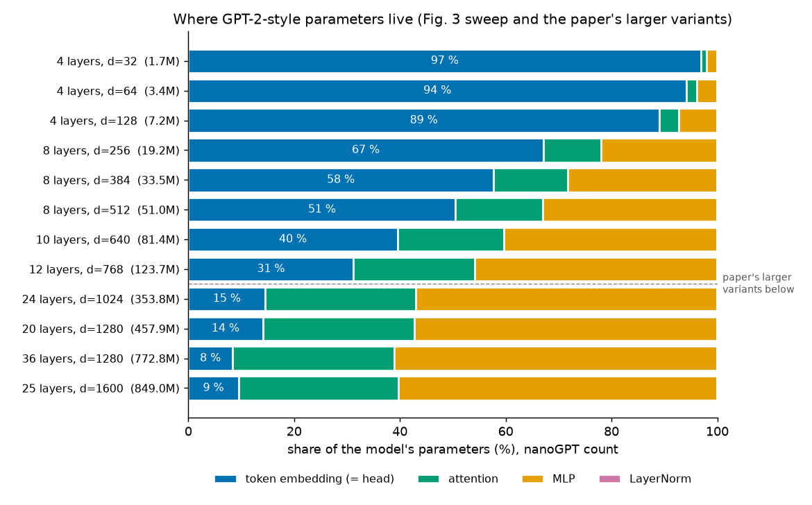
Figure: share of parameters by component, nanoGPT count. In the smallest model of Figure 3 the token embedding holds 96.9 % of all parameters; in GPT-2 small 31.2 %; in the 773M model 8.3 % (output [4]). The small models of the sweep are mostly a lookup table.
Paper erratum E24: Figure 3's parameter axis
PAPER Fig. 3, p. 8; App. E, p. 17 The figure gives no rule for its "Number of LLM Parameters".
MY EXPLANATION The x-positions are 1,895,722 … 124,753,293, read from the PDF by fig_extract.py. They are
counts with position embeddings and LoRA factors, while Table 3's labels (124M, 354M, …) are counts without
them. The same GPT-2-small shape is 123.69M in one convention and 124.75M in the other. No bound changes; only
the meaning of the axis.
Paper erratum E43: model sizes counted two ways, and two shapes never given
PAPER §6.4, p. 7; Table 3, p. 8; App. E, pp. 16–17 The paper names sizes 354M, 458M, 773M and 849M but gives shapes only through the names "GPT-2 medium" and "GPT-2 large". The shapes and head counts of 458M and 849M are never stated.
[SOURCE: authors' code, sublora_pipeline.py default bias=False; sublora/nn/model.py, read on GitHub, not in our saved sources] The released code
builds bias-free layers by default, except the fused query/key/value layer, which keeps a bias when LoRA is used.
MY ANALYSIS The labels follow nanoGPT's count with biases: without biases the 36 × 1,280 model has 772,271,360 parameters, which rounds to 772M, not 773M (output [3]). Figure 3 follows a third rule (all tensors of the bias-free LoRA model). No bound depends on these labels. A reader should still treat "773M" as a nominal size, not the exact count of the network that was trained.
Paper erratum E44: which attention matrices carry LoRA
PAPER §5, p. 6 §5 says LoRA is applied "only over the self-attention layer and the last linear layer". PAPER App. E, p. 16 Appendix E narrows this to the query and value matrices and the linear head.
MY EXPLANATION "Self-attention layer" could also include \(W_K\) and \(W_O\). Appendix E is the precise
statement. [SOURCE: authors' code, sublora/nn/model.py, read on GitHub, not in our saved sources] The code enables LoRA on query and value only
(enable_lora=[True, False, True]). The Figure 3 counts above agree to within 5.3 parts per million only with
this choice.
Going deeper¶
This chapter's proofs sit in the blocks below.
Going deeper: attention in matrix form, and why divide by the square root of d_head
MY EXPLANATION Put the normalized stream vectors as the rows of \(U\in\mathbb R^{T\times d_{\text{model}}}\). For one head, let \(\mathcal Q=UW_Q^\top\), \(\mathcal K=UW_K^\top\), \(\mathcal V=UW_V^\top\), each \(T\times d_{\text{head}}\) (row \(j\) is \(q_j^\top\), \(k_j^\top\), \(v_j^\top\)). Then all scores at once are
Add the mask matrix \(M\) with \(M_{ij}=0\) for \(j\le i\) and \(-\infty\) for \(j>i\), apply softmax to each row, and multiply by the values:
Cost: \(\mathcal Q\mathcal K^\top\) needs \(T^2d_{\text{head}}\) multiplications per head, so attention grows with the square of the number of tokens. That is one reason the context window is limited to \(L_{\text{ctx}}=1024\).
Why \(\sqrt{d_{\text{head}}}\). Suppose, as at the start of training, the entries of \(q_i\) and \(k_j\) are independent random variables with mean 0 and variance 1 (what is random: the entries; \(d_{\text{head}}\) is fixed). Then \(q_i\cdot k_j=\sum_{l=1}^{d_{\text{head}}}q_{il}k_{jl}\) is a sum of \(d_{\text{head}}\) independent terms. Each term has mean \(\mathbb E[q_{il}]\,\mathbb E[k_{jl}]=0\) and variance \(\mathbb E[q_{il}^2]\,\mathbb E[k_{jl}^2]=1\) (independence; Chapter 1). Variances of independent terms add (Chapter 8, deeper block on Gaussian matrices), so
Without the division, scores for \(d_{\text{head}}=64\) would have standard deviation 8. Softmax of such spread-out numbers puts almost all weight on one position, and small changes in the scores would barely change the weights. The division keeps scores of order 1 for every head size.
Weights are a proper average. Each row of \(\mathrm{softmax}(S+M)\) has positive entries for \(j\le i\), zero entries for \(j>i\) (because \(e^{-\infty}=0\)), and sums to 1 (softmax property, Chapter 4). So each output \(o_i\) is a convex combination (a weighted average with non-negative weights summing to 1) of \(v_1,\dots,v_i\). Every coordinate of \(o_i\) lies between the smallest and largest value of that coordinate among \(v_1,\dots,v_i\).
Going deeper: proof that the whole model is causal
MY EXPLANATION Claim: for every block \(\ell\) and position \(i\), the stream vector \(y_i^{(\ell)}\) depends only on the tokens \(x_1,\dots,x_i\). Hence the logits \(z^{(i)}\), and the distribution for token \(i+1\), depend only on \(x_{\le i}\), exactly what an autoregressive model (Chapter 4) requires.
Proof by induction on \(\ell\). For \(\ell=0\), \(y_i^{(0)}=W_E[x_i]+W_{\text{pos}}[i]\) uses only \(x_i\).
Assume the claim for \(\ell-1\). In block \(\ell\):
- \(\mathrm{LN}_1\) acts on each position separately, so \(\mathrm{LN}_1(y_j^{(\ell-1)})\) depends on \(x_{\le j}\).
- Queries, keys and values at \(j\) are matrix products of that vector, so they depend on \(x_{\le j}\).
- The output at \(i\) uses \(q_i\) and \(k_j,v_j\) for \(j\le i\) only, because the mask makes \(a_{ij}=0\) for \(j>i\). All of these depend on \(x_{\le i}\). Stacking heads and multiplying by \(W_O\) keeps this.
- The residual add, \(\mathrm{LN}_2\) and the MLP act on position \(i\) alone.
So \(y_i^{(\ell)}\) depends on \(x_{\le i}\). The final LayerNorm and the head act per position. \(\blacksquare\)
The script checks this numerically: changing token 9 leaves the logits at positions 1–8 exactly unchanged
(output [3] of ch05_attention.py).
One consequence matters for the paper. A single forward pass over a document of \(T\le L_{\text{ctx}}\) tokens yields all \(T\) next-token distributions at once, so the per-token losses of a whole document cost one pass.
Going deeper: layer normalization, precisely
MY EXPLANATION For \(u\in\mathbb R^{n}\) (\(n=d_{\text{model}}\)) let \(\mu=\frac1n\sum_ju_j\) and \(\sigma^2=\frac1n\sum_j(u_j-\mu)^2\), and set \(\hat u_j=(u_j-\mu)/\sigma\) (take \(\varepsilon=0\) and \(\sigma>0\)). Then
So the normalized vector has entry average 0 and entry variance 1, whatever the scale of \(u\). Note that \(\mu\) and \(\sigma\) are averages over the entries of one vector, not over a dataset; nothing here is random.
Two consequences. (i) \(\mathrm{LN}(cu)=\mathrm{LN}(u)\) for every \(c>0\): the stream can grow as blocks keep adding to it, but each block reads a vector of fixed scale. (ii) LayerNorm is not linear; it is one of the non-linear steps of the network, alongside GELU and softmax.
With \(\varepsilon>0\), the variance becomes \(\sigma^2/(\sigma^2+\varepsilon)\), slightly below 1; with \(\varepsilon=10^{-5}\) and \(\sigma^2\) of order 1 the difference is negligible.
Going deeper: the general parameter count, and why heads do not change it
MY EXPLANATION Write \(n=d_{\text{model}}\). One block contains:
| Piece | Weights | Biases / LayerNorm |
|---|---|---|
| \(W_Q,W_K,W_V\) | \(n\times3n=3n^2\) | \(3n\) |
| \(W_O\) | \(n\times n=n^2\) | \(n\) |
| MLP up | \(n\times4n=4n^2\) | \(4n\) |
| MLP down | \(4n\times n=4n^2\) | \(n\) |
| two LayerNorms | — | \(2\times2n=4n\) |
| sum | \(12n^2\) | \(13n\) |
The whole model, in nanoGPT's convention (padded vocabulary \(V_{\text{pad}}=50{,}304\), tied head, no position embedding, final LayerNorm \(2n\)):
Adding the position embedding adds \(L_{\text{ctx}}\,n\). Without biases, each block has \(12n^2+2n\) and the final LayerNorm \(n\).
Heads do not change the count. Head \(h\) has its own \(W_Q^{(h)}\in\mathbb R^{d_{\text{head}}\times n}\). Stacking the \(n_{\text{head}}\) head matrices gives one matrix of shape \((n_{\text{head}}d_{\text{head}})\times n=n\times n\), whatever \(n_{\text{head}}\) is. The same holds for keys and values, and \(W_O\) is \(n\times n\) in any case. So \((12,12,768)\) and a hypothetical \((12,6,768)\) have identical counts. This is why the head counts of the 458M and 849M models cannot be recovered from their sizes.
Multi-head attention as one big matrix product. Stacking the head outputs \(o_i^{(1)},\dots,o_i^{(n_{\text{head}})}\) into one vector and multiplying by \(W_O\) equals \(\sum_hW_O^{(h)}o_i^{(h)}\), where \(W_O^{(h)}\) is the block of \(d_{\text{head}}\) columns of \(W_O\) that meets head \(h\) (block multiplication, Chapter 8). The heads are separate only in how their weights \(a_{ij}\) are computed.
The LoRA factors (Chapter 19 defines LoRA; here we only count). A rank-\(r\) correction \(BA\) to a matrix of shape \(a\times b\) stores \(r(a+b)\) numbers (Chapter 8). On \(W_Q\) and \(W_V\) of every block that is \(2\cdot r(n+n)=4rn\) per block; on the head (\(V_{\text{pad}}\times n\)) it is \(r(V_{\text{pad}}+n)\). For GPT-2 small at \(r=4\): \(12\cdot4\cdot4\cdot768+4\cdot(50{,}304+768)=351{,}744\) (output [2]).
The authors' convention. [SOURCE: authors' code, sublora/nn/model.py, read on GitHub, not in our saved sources] get_num_params there sums
all parameter tensors (position embedding included). The layers are bias-free by default, but the fused
c_attn layer is created through the LoRA library without a bias argument and so keeps a bias of \(3n\).
MY EXPLANATION The count becomes
For \((12,12,768)\), \(r=4\), this is 124,753,152 against Figure 3's 124,753,293 (+1.1 parts per million; output [4]). The torch cross-check builds every shape on PyTorch's "meta" device (shapes only, no memory) and confirms both formulas exactly (output [5]).
Going deeper: other names for the same models (117M, 345M, 355M, 774M)
MY EXPLANATION Other sources label the four GPT-2 sizes differently. The labels below are the ones commonly quoted; this explainer did not check them against the original documents (the GPT-2 paper by Radford et al. 2019 and OpenAI's released checkpoints are not among our saved sources). The GPT-2 paper is commonly quoted as printing 117M, 345M, 762M and 1542M, and OpenAI's released checkpoints as being named 124M, 355M, 774M and 1558M.
MY EXPLANATION Our script computes the count with the real vocabulary 50,257, tied head, and the position embedding included: 124.4M, 354.8M, 774.0M, 1557.6M (output [3]). These match the commonly quoted checkpoint names. The paper's 354M and 773M come from nanoGPT's count (padded vocabulary, no position embedding). Neither is an error; they are different bookkeeping rules for the same shapes. The older 117M/345M/762M labels, if quoted correctly, match none of these rules exactly.
Going deeper: how the weight-tied head scores tokens
MY EXPLANATION With \(W_{\text{head}}=W_E\), the logit of token \(v\) at position \(i\) is
the dot product of the final stream vector with the input vector of token \(v\). A large logit means "the final vector points in the direction of token \(v\)'s embedding". So one table serves twice: as the dictionary that turns tokens into vectors, and as the list of directions against which the output is compared.
Two practical consequences. First, the table holds \(V_{\text{pad}}\,d_{\text{model}}\) numbers, which is the largest single piece of a small model: 96.9 % of the (4, 4, 32) model and 31.2 % of GPT-2 small (output [4]). Second, putting LoRA "on the linear head" changes the output use of this table without changing its input use, since the correction is added only where the head is applied. Chapter 19 and Chapter 20 return to this.
Common misconceptions¶
- Misconception: "More attention heads means more parameters." — Actually: the query, key and value matrices of all heads together are always \(d_{\text{model}}\times d_{\text{model}}\); heads only split them into slices. The count depends on \(n_{\text{layer}}\) and \(d_{\text{model}}\) alone (deeper block), which is why the heads of the 458M and 849M models cannot be inferred.
- Misconception: "Attention picks the single most relevant earlier token." — Actually: it takes a weighted average of all allowed value vectors. In the worked example, token 3 used weights \((0.198,0.401,0.401)\) and output \((0.599,0.802)\), a mixture, not a copy.
- Misconception: "A transformer layer overwrites its input with a new representation." — Actually: each block adds to the residual stream. The vector keeps its shape (\(12\times32\) before and after four blocks in output [3]) and every block reads the sum of all earlier contributions.
- Misconception: "Most of a language model's parameters are in attention." — Actually: in GPT-2 small the MLPs hold 45.82 %, the embedding 31.23 % and attention 22.92 %; in the smallest Figure 3 model the embedding alone is 96.9 %.
- Misconception: "124M is the exact number of parameters of the model in the paper." — Actually: it is the rounded nanoGPT count of the shape (123,689,472, no position embedding, with biases). The authors' trained network is bias-free in most layers and carries LoRA factors; summing all its parameter tensors gives 124,753,152, which is what Figure 3 plots (output [4]).
- Misconception: "The model sees the next token when predicting it, because the whole document is fed in at once." — Actually: the causal mask makes every prediction depend only on earlier tokens; changing token 9 left positions 1–8 bit-for-bit unchanged (output [3]).
Self-test¶
Q1. Using nanoGPT's convention (padded vocabulary 50,304, biases, tied head, no position embedding), how many parameters does GPT-2 medium (24 layers, \(d_{\text{model}}=1{,}024\)) have? Does the answer change if it uses 8 heads instead of 16?
Answer
\(D=50{,}304\cdot1{,}024+24\,(12\cdot1{,}024^2+13\cdot1{,}024)+2\cdot1{,}024=353{,}822{,}720\), which rounds to the
paper's 354M (output [3] of ch05_param_count.py). The number of heads does not matter: the stacked query, key
and value matrices are \(1{,}024\times1{,}024\) each for any split into heads, so 8 heads give the same count.
Q2. In the three-token example, why is the first row of attention weights \((1,0,0)\) no matter what the queries and keys are? What would go wrong for a language model without this?
Answer
The causal mask sets the scores for \(j=2,3\) to \(-\infty\), and \(e^{-\infty}=0\), so softmax puts all weight on the only allowed position, \(j=1\). Without the mask, token 1's vector would mix in information from tokens 2 and 3 (weights \((0.401,0.198,0.401)\) in the example). Its logits, which are supposed to predict token 2, would then depend on token 2 itself. The model would score the training text using the answers, and its probabilities would no longer factor as a chain of next-token predictions (Chapter 4).
Q3. Figure 3's smallest point sits at 1,895,722 parameters, but nanoGPT's count for (4, 4, 32) is 1,660,608. Account for the difference.
Answer
Figure 3 counts every parameter tensor of the trained model. Start from the bias-free base \(50{,}304\cdot32+4\,(12\cdot32^2+2\cdot32)+32=1{,}659{,}168\) and add the position embedding (\(1{,}024\cdot32=32{,}768\)), the bias of the fused query/key/value layer (\(4\cdot3\cdot32=384\)), rank-4 LoRA on \(W_Q\) and \(W_V\) (\(4\cdot4\cdot4\cdot32=2{,}048\)) and on the head (\(4\cdot(50{,}304+32)=201{,}344\)). The total is 1,895,712, which differs from the plotted 1,895,722 by 5.3 parts per million (output [4]). Most of the gap comes from LoRA on the head, whose \(50{,}304\times4\) factor is large next to such a small model.
Code for this chapter¶
Run them from the project root (each takes a few seconds on a laptop CPU):
.venv/Scripts/python explainer/code/ch05_param_count.py
.venv/Scripts/python explainer/code/ch05_attention.py
Source: ch05_param_count.py
"""Chapter 5 demo -- where the parameter counts of the paper's GPT-2 models come from.

Claims reproduced / checked (every number quoted in Chapter 5 about parameter counts is printed here):
  [1] GPT-2 small (12 layers, d = 768; PAPER App. E, p. 16) has 123,689,472 parameters in nanoGPT's
      convention (padded vocabulary 50,304, weight tying, position embedding excluded) -> "124M".
  [2] Share of those parameters in the token embedding, attention, MLP and LayerNorms.
  [3] The paper's sizes 354M (GPT-2 medium), 773M (GPT-2 large) follow the same convention; "458M" and
      "849M" are INFERRED (MY ANALYSIS) to be 20 x 1280 and 25 x 1600. Other counting conventions
      (OpenAI checkpoint names) are shown for comparison.
  [4] Figure 3's x-positions (read from the PDF by fig_extract.py) equal the parameter counts of the eight
      App. E sweep configurations counted WITH position embeddings and rank-4 LoRA factors on q, v and the
      head: within 0.09 % with pacbound's default (biased) layers, and within 10 parts per million with
      the authors' code (bias-free layers except the fused q/k/v projection; SOURCE: authors' code).
  [5] Cross-check of every formula by building the models in torch on the "meta" device and counting tensors.
Figure: explainer/docs/assets/fig/ch05_param_shares.png
Deterministic, CPU only, runs in a few seconds.
"""
from __future__ import annotations

import json
import sys
from pathlib import Path

import matplotlib

matplotlib.use("Agg")
import matplotlib.pyplot as plt  # noqa: E402
import torch  # noqa: E402
import torch.nn as nn  # noqa: E402

HERE = Path(__file__).resolve().parent
sys.path.insert(0, str(HERE))
import pacbound  # noqa: E402

OUT_TXT = HERE / "outputs" / "ch05_param_count.txt"
OUT_FIG = HERE.parent / "docs" / "assets" / "fig" / "ch05_param_shares.png"
FIG_JSON = HERE / "outputs" / "fig_extract.json"

V_PAD = 50304          # [SOURCE nanoGPT] 50,257 rounded up to a multiple of 64
V = pacbound.V_GPT2    # [SOURCE GPT-2 tokenizer] 50,257 (never printed in the paper, erratum E36)
CTX = pacbound.CONTEXT  # [PAPER App. E] 1024

_lines: list[str] = []


def out(s: str = "") -> None:
    print(s)
    _lines.append(s)


def pieces(d: int, vocab: int = V_PAD, bias: bool = True) -> dict:
    """Parameter count of every piece of one nanoGPT GPT-2 model (weights + biases), d = n_embd."""
    b = 1 if bias else 0
    return {
        "wte": vocab * d,                       # token embedding V x d (shared with the head)
        "wpe": CTX * d,                         # position embedding L_ctx x d
        "ln1": 2 * d if bias else d,            # LayerNorm before attention: gain (+ shift)
        "c_attn": d * 3 * d + b * 3 * d,        # W_Q, W_K, W_V side by side: d x 3d (+ 3d bias)
        "attn_proj": d * d + b * d,             # output projection W_O: d x d (+ d)
        "ln2": 2 * d if bias else d,            # LayerNorm before the MLP
        "c_fc": d * 4 * d + b * 4 * d,          # MLP up: d x 4d (+ 4d)
        "mlp_proj": 4 * d * d + b * d,          # MLP down: 4d x d (+ d)
        "ln_f": 2 * d if bias else d,           # final LayerNorm
    }


def block_total(p: dict) -> int:
    return p["ln1"] + p["c_attn"] + p["attn_proj"] + p["ln2"] + p["c_fc"] + p["mlp_proj"]


def lora_count(n_layer: int, d: int, r: int = 4, vocab: int = V_PAD) -> int:
    """Rank-r LoRA factors on W_Q and W_V of every layer (loralib MergedLinear, enable_lora=[T,F,T]:
    A is 2r x d, B is 2d x r) and on the head (A r x d, B vocab x r). [SOURCE: authors' code]"""
    return n_layer * (2 * r * d + 2 * d * r) + (r * d + vocab * r)


def authors_num_params(n_layer: int, d: int, r: int = 4, vocab: int = V_PAD) -> int:
    """What the authors' GPT.get_num_params() returns (sum of all parameter tensors):
    bias-free layers (code default bias=False) EXCEPT the LoRA c_attn (loralib MergedLinear keeps
    nn.Linear's default bias: +3d per layer), position embedding included, LoRA factors included.
    New helper (not in pacbound)."""
    return (pacbound.gpt2_params(n_layer, d, vocab=vocab, include_pos=True, bias=False)
            + 3 * d * n_layer + lora_count(n_layer, d, r, vocab))


# --------------------------------------------------------------------------- torch cross-check
class LN(nn.Module):
    def __init__(self, d, bias):
        super().__init__()
        self.weight = nn.Parameter(torch.ones(d))
        self.bias = nn.Parameter(torch.zeros(d)) if bias else None


class Block(nn.Module):
    def __init__(self, d, bias, attn_bias, r):
        super().__init__()
        self.ln_1, self.ln_2 = LN(d, bias), LN(d, bias)
        self.c_attn = nn.Linear(d, 3 * d, bias=attn_bias)
        self.attn_proj = nn.Linear(d, d, bias=bias)
        self.c_fc = nn.Linear(d, 4 * d, bias=bias)
        self.mlp_proj = nn.Linear(4 * d, d, bias=bias)
        if r:
            self.lora_A = nn.Parameter(torch.zeros(2 * r, d))
            self.lora_B = nn.Parameter(torch.zeros(2 * d, r))


class GPT(nn.Module):
    def __init__(self, n_layer, d, bias=True, attn_bias=True, r=0, vocab=V_PAD):
        super().__init__()
        self.wte = nn.Embedding(vocab, d)
        self.wpe = nn.Embedding(CTX, d)
        self.h = nn.ModuleList(Block(d, bias, attn_bias, r) for _ in range(n_layer))
        self.ln_f = LN(d, bias)
        self.lm_head = nn.Linear(d, vocab, bias=False)
        self.wte.weight = self.lm_head.weight          # weight tying (nanoGPT)
        if r:
            self.head_A = nn.Parameter(torch.zeros(r, d))
            self.head_B = nn.Parameter(torch.zeros(vocab, r))


def torch_count(model: nn.Module) -> int:
    return sum(p.numel() for p in model.parameters())   # shared (tied) tensors are counted once


def main() -> None:
    out("Chapter 5 -- parameter counts of the paper's GPT-2 models (ch05_param_count.py)")

    # [1] GPT-2 small by hand ---------------------------------------------------------------
    d, L = 768, 12
    p = pieces(d)
    out(f"[1] GPT-2 small, nanoGPT convention: L_layers = {L}, d = {d}, heads = 12 x {d // 12} dims, "
        f"MLP width 4d = {4 * d}")
    out(f"    token embedding 50,304 x 768            = {p['wte']:>12,}  (= the head, weight tying)")
    out(f"    per block: LayerNorm 1 (gain+shift 2d)  = {p['ln1']:>12,}")
    out(f"               W_Q,W_K,W_V  768 x 2304 + 2304 = {p['c_attn']:>12,}")
    out(f"               W_O          768 x 768 + 768   = {p['attn_proj']:>12,}")
    out(f"               LayerNorm 2                    = {p['ln2']:>12,}")
    out(f"               MLP up       768 x 3072 + 3072 = {p['c_fc']:>12,}")
    out(f"               MLP down     3072 x 768 + 768  = {p['mlp_proj']:>12,}")
    bt = block_total(p)
    out(f"    one block = 12 d^2 + 13 d = {12 * d * d:,} + {13 * d:,} = {bt:,};  x 12 blocks = {L * bt:,}")
    total = p["wte"] + L * bt + p["ln_f"]
    out(f"    final LayerNorm = {p['ln_f']:,};  TOTAL = {total:,}  -> rounds to {round(total / 1e6)}M")
    out(f"    (not counted: position embedding 1024 x 768 = {p['wpe']:,}; padding rows 50,304 - 50,257 = "
        f"{V_PAD - V} -> {(V_PAD - V) * d:,} unused numbers)")
    assert total == pacbound.gpt2_params(L, d) == 123_689_472 and bt == 7_087_872

    # [2] shares ----------------------------------------------------------------------------
    att = L * (p["c_attn"] + p["attn_proj"])
    mlp = L * (p["c_fc"] + p["mlp_proj"])
    lns = L * (p["ln1"] + p["ln2"]) + p["ln_f"]
    assert p["wte"] + att + mlp + lns == total
    out("[2] Where GPT-2 small's 123,689,472 parameters live:")
    out(f"    token embedding {p['wte']:>11,} = {100 * p['wte'] / total:5.2f} %   attention {att:>11,} = "
        f"{100 * att / total:5.2f} %")
    out(f"    MLPs            {mlp:>11,} = {100 * mlp / total:5.2f} %   LayerNorms {lns:>10,} = "
        f"{100 * lns / total:5.3f} %")
    lq = lora_count(L, d, 4)
    out(f"    rank-4 LoRA on W_Q, W_V and head would add {lq:,} = {100 * lq / total:.3f} % "
        f"(W_Q and W_V of one layer: 2 x 768 x 768 = {2 * d * d:,})")
    lq_true = lora_count(L, d, 4, vocab=V)
    assert lq - lq_true == 4 * (V_PAD - V)
    out(f"    (that uses nanoGPT's padded head, V = {V_PAD:,}; with the true V = {V:,} it is {lq_true:,}, "
        f"{lq - lq_true} fewer = 4 x {V_PAD - V})")

    # [3] the paper's model sizes -----------------------------------------------------------
    out("[3] Paper sizes (§6.4, Table 3, App. E) vs nanoGPT count (biases, no position embedding, V = 50,304)")
    rows = [("124M", 12, 768, "12", "given in App. E"),
            ("354M", 24, 1024, "16", "GPT-2 medium [SOURCE]"),
            ("458M", 20, 1280, "?", "INFERRED (MY ANALYSIS)"),
            ("773M", 36, 1280, "20", "GPT-2 large [SOURCE]"),
            ("849M", 25, 1600, "?", "INFERRED (MY ANALYSIS)")]
    out("    label  layers x d    heads  count           rounds   same, bias-free   rounds")
    for lab, nl, dd, hh, note in rows:
        c = pacbound.gpt2_params(nl, dd)
        cf = pacbound.gpt2_params(nl, dd, bias=False)
        out(f"    {lab:>5}  {nl:>3} x {dd:<5}  {hh:>5}  {c:>13,}  {round(c / 1e6):>4}M   {cf:>13,}  "
            f"{round(cf / 1e6):>4}M   {note}")
        assert f"{round(c / 1e6)}M" == lab
    gpt2_widths = [768, 1024, 1280, 1600]
    for lab in ("458M", "849M"):
        t = int(lab[:-1])
        cand = [(nl, dd) for dd in gpt2_widths for nl in range(1, 97)
                if round(pacbound.gpt2_params(nl, dd) / 1e6) == t]
        cand64 = [(nl, dd) for dd in range(64, 4097, 64) for nl in range(1, 97)
                  if round(pacbound.gpt2_params(nl, dd) / 1e6) == t]
        fam = [nl for nl in range(1, 97) if round(pacbound.gpt2_params(nl, 64 * nl) / 1e6) == t]
        out(f"    {lab}: shapes with a GPT-2 width (768/1024/1280/1600): {cand};  any width that is a "
            f"multiple of 64: {len(cand64)};  family d = 64 x layers: layers = {fam}")
    assert pacbound.gpt2_params(20, 1280) == 457_940_480 and pacbound.gpt2_params(25, 1600) == 849_009_600
    oa = [(12, 768), (24, 1024), (36, 1280), (48, 1600)]
    oac = [pacbound.gpt2_params(nl, dd, vocab=V, include_pos=True) for nl, dd in oa]
    out("    OpenAI checkpoint convention (V = 50,257, position embedding counted): "
        + ", ".join(f"{c / 1e6:.1f}M" for c in oac))
    out("      -> matches the commonly quoted checkpoint names 124M, 355M, 774M, 1558M (openai/gpt-2;"
        " GPT-2 paper commonly quoted as 117M, 345M, 762M, 1542M; not checked against saved sources)")
    assert [round(c / 1e6) for c in oac] == [124, 355, 774, 1558]

    # [4] Figure 3 x-positions ----------------------------------------------------------------
    sweep = [(4, 4, 32), (4, 4, 64), (4, 4, 128), (8, 8, 256), (8, 8, 384), (8, 8, 512),
             (10, 10, 640), (12, 12, 768)]                       # [PAPER App. E, p. 17]
    fig_x = [1895722, 3688527, 7569052, 19676969, 34133447, 51735630, 82340777, 124753293]
    if FIG_JSON.exists():
        js = json.loads(FIG_JSON.read_text(encoding="utf-8"))
        assert [pt["params"] for pt in js["figure3"]["bpd_bound"]["best_line"]] == fig_x
    out("[4] Figure 3 x-positions (fig_extract.py) vs counts with position embedding + rank-4 LoRA (q, v, head)")
    out("    (layers,heads,d)  nanoGPT count   +pos+LoRA (pacbound)  diff     authors' count   Fig. 3 x       diff")
    worst_a, worst_b = 0.0, 0.0
    for (nl, nh, dd), x in zip(sweep, fig_x):
        c0 = pacbound.gpt2_params(nl, dd)
        ca = pacbound.gpt2_params(nl, dd, include_pos=True) + lora_count(nl, dd, 4)
        cb = authors_num_params(nl, dd, 4)
        ra, rb = x / ca - 1, x / cb - 1
        worst_a, worst_b = max(worst_a, abs(ra)), max(worst_b, abs(rb))
        out(f"    ({nl:>2},{nh:>2},{dd:>4})  {c0:>13,}  {ca:>13,}  {100 * ra:+7.3f} %  {cb:>13,}  {x:>13,}  "
            f"{1e6 * rb:+5.1f} ppm")
    out(f"    largest mismatch: {100 * worst_a:.3f} % (pacbound, biased layers);  {1e6 * worst_b:.1f} ppm "
        f"(authors' code convention)")
    nl, dd = 4, 32
    base = pacbound.gpt2_params(nl, dd, bias=False)
    out(f"    (4,4,32) authors' count = bias-free base {base:,} + position emb. {CTX * dd:,} + c_attn bias "
        f"{3 * dd * nl:,} + LoRA q,v {nl * 4 * 4 * dd:,} + LoRA head {4 * (dd + V_PAD):,} = "
        f"{authors_num_params(nl, dd):,}")
    alt = max(abs(x / pacbound.gpt2_params(nl, dd) - 1) for (nl, nh, dd), x in zip(sweep, fig_x))
    out(f"    without position embedding and LoRA the mismatch reaches {100 * alt:.1f} % (smallest model)")
    assert worst_a < 1e-3 and worst_b < 1e-5
    pct = [round(pacbound.gpt2_params(nl, dd) / 1e6, 2) for nl, nh, dd in sweep]
    out("    nanoGPT counts in millions: " + ", ".join(f"{v:g}" for v in pct))
    emb = [100 * V_PAD * dd / pacbound.gpt2_params(nl, dd) for nl, dd in
           [(nl, dd) for nl, _, dd in sweep] + [(24, 1024), (20, 1280), (36, 1280), (25, 1600)]]
    out("    token-embedding share (%), 8 sweep models then 354M/458M/773M/849M: "
        + ", ".join(f"{e:.1f}" for e in emb))

    # [5] torch cross-check ---------------------------------------------------------------------
    shapes = sorted({(nl, dd) for nl, _, dd in sweep} | {(nl, dd) for _, nl, dd, _, _ in rows})
    n_ok = 0
    with torch.device("meta"):
        for nl, dd in shapes:
            m1 = GPT(nl, dd, bias=True, attn_bias=True, r=0)
            assert torch_count(m1) - m1.wpe.weight.numel() == pacbound.gpt2_params(nl, dd)
            m2 = GPT(nl, dd, bias=False, attn_bias=True, r=4)
            assert torch_count(m2) == authors_num_params(nl, dd, 4)
            n_ok += 1
        untied = GPT(12, 768)
        untied.wte.weight = nn.Parameter(torch.empty(V_PAD, 768))
        extra = torch_count(untied) - torch_count(GPT(12, 768))
    out(f"[5] torch (meta device) counts agree with both formulas for all {n_ok} shapes; "
        f"untying the head would add {extra:,} parameters")

    # figure ------------------------------------------------------------------------------------
    cfgs = [(nl, dd) for nl, _, dd in sweep] + [(24, 1024), (20, 1280), (36, 1280), (25, 1600)]
    labels, shares = [], []
    for nl, dd in cfgs:
        q = pieces(dd)
        tot = pacbound.gpt2_params(nl, dd)
        parts = [q["wte"], nl * (q["c_attn"] + q["attn_proj"]), nl * (q["c_fc"] + q["mlp_proj"]),
                 nl * (q["ln1"] + q["ln2"]) + q["ln_f"]]
        assert sum(parts) == tot
        shares.append([100 * x / tot for x in parts])
        labels.append(f"{nl} layers, d={dd}  ({tot / 1e6:.1f}M)")
    names = ["token embedding (= head)", "attention", "MLP", "LayerNorm"]
    cols = ["#0072B2", "#009E73", "#E69F00", "#CC79A7"]
    fig, ax = plt.subplots(figsize=(9.0, 5.6))
    ys = list(range(len(cfgs)))[::-1]
    for i, (y, sh) in enumerate(zip(ys, shares)):
        left = 0.0
        for j, s in enumerate(sh):
            ax.barh(y, s, left=left, color=cols[j], edgecolor="white", linewidth=1.5,
                    label=names[j] if i == 0 else None)
            left += s
        ax.text(sh[0] / 2, y, f"{sh[0]:.0f} %", ha="center", va="center", color="white", fontsize=9)
    ax.axhline(3.5, color="#888888", lw=0.8, ls="--")
    ax.text(101, 3.5, "paper's larger\nvariants below", fontsize=8, va="center", color="#555555")
    ax.set_yticks(ys)
    ax.set_yticklabels(labels, fontsize=9)
    ax.set_xlim(0, 100)
    ax.set_xlabel("share of the model's parameters (%), nanoGPT count")
    ax.set_title("Where GPT-2-style parameters live (Fig. 3 sweep and the paper's larger variants)", fontsize=11)
    ax.legend(loc="upper center", bbox_to_anchor=(0.5, -0.12), ncol=4, fontsize=9, frameon=False)
    for s in ("top", "right"):
        ax.spines[s].set_visible(False)
    fig.tight_layout()
    OUT_FIG.parent.mkdir(parents=True, exist_ok=True)
    fig.savefig(OUT_FIG, dpi=130)
    out(f"figure: docs/assets/fig/{OUT_FIG.name}. All assertions passed.")

    OUT_TXT.parent.mkdir(parents=True, exist_ok=True)
    OUT_TXT.write_text("\n".join(_lines) + "\n", encoding="utf-8")


if __name__ == "__main__":
    main()
Output of ch05_param_count.py:
Chapter 5 -- parameter counts of the paper's GPT-2 models (ch05_param_count.py)
[1] GPT-2 small, nanoGPT convention: L_layers = 12, d = 768, heads = 12 x 64 dims, MLP width 4d = 3072
    token embedding 50,304 x 768            =   38,633,472  (= the head, weight tying)
    per block: LayerNorm 1 (gain+shift 2d)  =        1,536
               W_Q,W_K,W_V  768 x 2304 + 2304 =    1,771,776
               W_O          768 x 768 + 768   =      590,592
               LayerNorm 2                    =        1,536
               MLP up       768 x 3072 + 3072 =    2,362,368
               MLP down     3072 x 768 + 768  =    2,360,064
    one block = 12 d^2 + 13 d = 7,077,888 + 9,984 = 7,087,872;  x 12 blocks = 85,054,464
    final LayerNorm = 1,536;  TOTAL = 123,689,472  -> rounds to 124M
    (not counted: position embedding 1024 x 768 = 786,432; padding rows 50,304 - 50,257 = 47 -> 36,096 unused numbers)
[2] Where GPT-2 small's 123,689,472 parameters live:
    token embedding  38,633,472 = 31.23 %   attention  28,348,416 = 22.92 %
    MLPs             56,669,184 = 45.82 %   LayerNorms     38,400 = 0.031 %
    rank-4 LoRA on W_Q, W_V and head would add 351,744 = 0.284 % (W_Q and W_V of one layer: 2 x 768 x 768 = 1,179,648)
    (that uses nanoGPT's padded head, V = 50,304; with the true V = 50,257 it is 351,556, 188 fewer = 4 x 47)
[3] Paper sizes (§6.4, Table 3, App. E) vs nanoGPT count (biases, no position embedding, V = 50,304)
    label  layers x d    heads  count           rounds   same, bias-free   rounds
     124M   12 x 768       12    123,689,472   124M     123,587,328   124M   given in App. E
     354M   24 x 1024      16    353,822,720   354M     353,551,360   354M   GPT-2 medium [SOURCE]
     458M   20 x 1280       ?    457,940,480   458M     457,657,600   458M   INFERRED (MY ANALYSIS)
     773M   36 x 1280      20    772,779,520   773M     772,271,360   772M   GPT-2 large [SOURCE]
     849M   25 x 1600       ?    849,009,600   849M     848,568,000   849M   INFERRED (MY ANALYSIS)
    458M: shapes with a GPT-2 width (768/1024/1280/1600): [(20, 1280)];  any width that is a multiple of 64: 5;  family d = 64 x layers: layers = [20]
    849M: shapes with a GPT-2 width (768/1024/1280/1600): [(25, 1600)];  any width that is a multiple of 64: 3;  family d = 64 x layers: layers = [25]
    OpenAI checkpoint convention (V = 50,257, position embedding counted): 124.4M, 354.8M, 774.0M, 1557.6M
      -> matches the commonly quoted checkpoint names 124M, 355M, 774M, 1558M (openai/gpt-2; GPT-2 paper commonly quoted as 117M, 345M, 762M, 1542M; not checked against saved sources)
[4] Figure 3 x-positions (fig_extract.py) vs counts with position embedding + rank-4 LoRA (q, v, head)
    (layers,heads,d)  nanoGPT count   +pos+LoRA (pacbound)  diff     authors' count   Fig. 3 x       diff
    ( 4, 4,  32)      1,660,608      1,896,768   -0.055 %      1,895,712      1,895,722   +5.3 ppm
    ( 4, 4,  64)      3,419,520      3,690,624   -0.057 %      3,688,512      3,688,527   +4.1 ppm
    ( 4, 4, 128)      7,232,256      7,573,248   -0.055 %      7,569,024      7,569,052   +3.7 ppm
    ( 8, 8, 256)     19,196,416     19,693,568   -0.084 %     19,676,928     19,676,969   +2.1 ppm
    ( 8, 8, 384)     33,513,216     34,158,336   -0.073 %     34,133,376     34,133,447   +2.1 ppm
    ( 8, 8, 512)     50,975,744     51,768,832   -0.064 %     51,735,552     51,735,630   +1.5 ppm
    (10,10, 640)     81,431,040     82,392,576   -0.063 %     82,340,736     82,340,777   +0.5 ppm
    (12,12, 768)    123,689,472    124,827,648   -0.060 %    124,753,152    124,753,293   +1.1 ppm
    largest mismatch: 0.084 % (pacbound, biased layers);  5.3 ppm (authors' code convention)
    (4,4,32) authors' count = bias-free base 1,659,168 + position emb. 32,768 + c_attn bias 384 + LoRA q,v 2,048 + LoRA head 201,344 = 1,895,712
    without position embedding and LoRA the mismatch reaches 14.2 % (smallest model)
    nanoGPT counts in millions: 1.66, 3.42, 7.23, 19.2, 33.51, 50.98, 81.43, 123.69
    token-embedding share (%), 8 sweep models then 354M/458M/773M/849M: 96.9, 94.1, 89.0, 67.1, 57.6, 50.5, 39.5, 31.2, 14.6, 14.1, 8.3, 9.5
[5] torch (meta device) counts agree with both formulas for all 12 shapes; untying the head would add 38,633,472 parameters
figure: docs/assets/fig/ch05_param_shares.png. All assertions passed.
Source: ch05_attention.py
"""Chapter 5 demo -- the arithmetic inside one transformer block, on numbers small enough to check by hand.

Claims reproduced / checked (every number in Chapter 5's worked attention example is printed here):
  [1] GELU and layer normalization on tiny vectors.
  [2] Causal self-attention for 3 tokens with d_head = 2: scores q.k / sqrt(d_head), causal mask, softmax
      weights (each row sums to 1), weighted averages of the value vectors.
  [3] A real (randomly initialized) GPT-2-style model with 4 layers, 4 heads, d = 32 (the smallest model
      of the paper's Figure 3 sweep, App. E p. 17), built in torch on the CPU:
      shapes along the residual stream, logits of size 50,304 per position, causality (changing a later
      token never changes earlier predictions), and the untrained model's surprisal ~ log2 V bits/token.
Deterministic (torch.manual_seed(0)); CPU only; runs in a few seconds.
"""
from __future__ import annotations

import math
import sys
from pathlib import Path

import numpy as np
import torch
import torch.nn as nn
import torch.nn.functional as F

HERE = Path(__file__).resolve().parent
sys.path.insert(0, str(HERE))
import pacbound  # noqa: E402

OUT_TXT = HERE / "outputs" / "ch05_attention.txt"
V_PAD = 50304
_lines: list[str] = []


def out(s: str = "") -> None:
    print(s)
    _lines.append(s)


def vec(a) -> str:
    return "(" + ", ".join(f"{x:.3f}" for x in a) + ")"


def gelu(x: float) -> float:
    return 0.5 * x * (1.0 + math.erf(x / math.sqrt(2.0)))


# --------------------------------------------------------------------------- tiny GPT (nanoGPT layout)
class Block(nn.Module):
    def __init__(self, d: int, n_head: int):
        super().__init__()
        self.h, self.d = n_head, d
        self.ln_1, self.ln_2 = nn.LayerNorm(d), nn.LayerNorm(d)
        self.c_attn = nn.Linear(d, 3 * d)       # W_Q, W_K, W_V side by side
        self.attn_proj = nn.Linear(d, d)        # W_O
        self.c_fc = nn.Linear(d, 4 * d)
        self.mlp_proj = nn.Linear(4 * d, d)

    def attention(self, x):
        T, d, H = x.shape[0], self.d, self.h
        q, k, v = self.c_attn(x).split(d, dim=1)                     # each T x d
        q, k, v = (t.view(T, H, d // H).transpose(0, 1) for t in (q, k, v))   # H x T x d_head
        s = q @ k.transpose(1, 2) / math.sqrt(d // H)                 # H x T x T scores
        mask = torch.triu(torch.ones(T, T, dtype=torch.bool), diagonal=1)
        a = F.softmax(s.masked_fill(mask, float("-inf")), dim=-1)    # causal attention weights
        self.last_weights = a
        y = (a @ v).transpose(0, 1).reshape(T, d)                     # concatenate the heads
        return self.attn_proj(y)

    def forward(self, x):
        x = x + self.attention(self.ln_1(x))                           # residual add 1
        x = x + self.mlp_proj(F.gelu(self.c_fc(self.ln_2(x))))         # residual add 2
        return x


class TinyGPT(nn.Module):
    def __init__(self, n_layer=4, n_head=4, d=32, ctx=1024):
        super().__init__()
        self.wte, self.wpe = nn.Embedding(V_PAD, d), nn.Embedding(ctx, d)
        self.blocks = nn.ModuleList(Block(d, n_head) for _ in range(n_layer))
        self.ln_f = nn.LayerNorm(d)
        self.lm_head = nn.Linear(d, V_PAD, bias=False)
        self.wte.weight = self.lm_head.weight                         # weight tying
        for name, p in self.named_parameters():                       # nanoGPT initialization
            if p.dim() == 2:
                std = 0.02 / math.sqrt(2 * n_layer) if name.endswith("proj.weight") else 0.02
                nn.init.normal_(p, 0.0, std)
            elif name.endswith("bias"):
                nn.init.zeros_(p)

    def forward(self, idx):
        x = self.wte(idx) + self.wpe(torch.arange(idx.shape[0]))      # residual stream, T x d
        self.stream_shapes = [tuple(x.shape)]
        for b in self.blocks:
            x = b(x)
            self.stream_shapes.append(tuple(x.shape))
        return self.lm_head(self.ln_f(x))                              # logits, T x V_PAD


def main() -> None:
    out("Chapter 5 -- inside a transformer block (ch05_attention.py)")

    # [1] GELU and LayerNorm -------------------------------------------------------------------
    out("[1] GELU(x) = x * Phi(x):  " + ",  ".join(f"GELU({x:g}) = {gelu(x):.4f}" for x in (-2, -1, 0, 1, 2)))
    x = np.array([1.0, 2.0, 3.0, 6.0])
    mu, var = x.mean(), x.var()
    z = (x - mu) / np.sqrt(var)
    out(f"    LayerNorm of x = (1, 2, 3, 6): mean {mu:g}, variance {var:g}, std {np.sqrt(var):.4f} -> "
        f"{vec(z)}  (new mean {abs(z.mean()):.0f}, new variance {z.var():.4f})")

    # [2] three-token causal attention ---------------------------------------------------------
    q = np.array([[1.0, 0.0], [0.0, 1.0], [1.0, 1.0]])
    k = np.array([[1.0, 0.0], [0.0, 2.0], [1.0, 1.0]])
    v = np.array([[1.0, 0.0], [0.0, 1.0], [1.0, 1.0]])
    dh = q.shape[1]
    raw = q @ k.T
    s = raw / math.sqrt(dh)
    masked = np.where(np.triu(np.ones((3, 3), bool), 1), -np.inf, s)
    w = np.exp(masked - masked.max(axis=1, keepdims=True))
    w = w / w.sum(axis=1, keepdims=True)
    o = w @ v
    out(f"[2] Three tokens, d_head = {dh}, sqrt(d_head) = {math.sqrt(dh):.4f}")
    for i in range(3):
        out(f"    token {i + 1}: q = {vec(q[i])}  k = {vec(k[i])}  v = {vec(v[i])}")
    for i in range(3):
        out(f"    row {i + 1}: q.k = {vec(raw[i])}  scaled = {vec(s[i])}  after mask = "
            + "(" + ", ".join("-inf" if np.isinf(t) else f"{t:.3f}" for t in masked[i]) + ")")
    for i in range(3):
        out(f"    row {i + 1}: weights = {vec(w[i])} (sum {w[i].sum():.3f})  output = {vec(o[i])}")
    nm = np.exp(s[0] - s[0].max())
    out(f"    without the mask, token 1 would use weights {vec(nm / nm.sum())} -- it would see the future")
    assert np.allclose(w.sum(axis=1), 1) and np.all(w[np.triu_indices(3, 1)] == 0)
    a, b = math.exp(1 / math.sqrt(2)), math.exp(2 / math.sqrt(2))       # hand formula for row 3
    assert np.allclose(o[2], [(a + b) / (a + 2 * b), 2 * b / (a + 2 * b)])

    # [3] a real tiny GPT ---------------------------------------------------------------------
    torch.manual_seed(0)
    model = TinyGPT()
    n_all = sum(p.numel() for p in model.parameters())
    n_conv = n_all - model.wpe.weight.numel()
    assert n_conv == pacbound.gpt2_params(4, 32)
    T = 12
    idx = torch.randint(0, 50257, (T,))
    with torch.no_grad():
        logits = model(idx)
        attw = model.blocks[0].last_weights
        idx2 = idx.clone()
        idx2[8] = (idx2[8] + 1) % 50257
        logits2 = model(idx2)
        lp = F.log_softmax(logits, dim=-1)
        surpr = -lp[:-1].gather(1, idx[1:, None]).squeeze(1) / math.log(2)   # bits/token
    diff = (logits2 - logits).abs().amax(dim=1)
    out(f"[3] Tiny GPT (4 layers, 4 heads, d = 32, seed 0): {n_conv:,} parameters (nanoGPT count), "
        f"{n_all:,} with the position embedding")
    out(f"    {T} tokens in -> residual stream {model.stream_shapes[0]} after embedding, "
        f"{model.stream_shapes[-1]} after 4 blocks -> logits {tuple(logits.shape)}")
    out(f"    attention weights, layer 1: shape {tuple(attw.shape)} (heads x T x T); largest row-sum error "
        f"{(attw.sum(-1) - 1).abs().max().item():.1e}; weight above the diagonal = {attw.triu(1).abs().max().item():g}")
    out(f"    change token 9 only: max |change| of logits at positions 1-8 = {diff[:8].max().item():g}, "
        f"at positions 9-12 = {diff[8:].min().item():.3g} ... {diff[8:].max().item():.3g}")
    out(f"    untrained model: mean surprisal of the next token = {surpr.mean().item():.3f} bits/token "
        f"(log2 50,304 = {math.log2(V_PAD):.3f}; log2 V = log2 50,257 = {pacbound.random_guess_bpd():.3f})")
    out(f"    softmax over all 50,304 logits sums to {lp.exp().sum(-1).mean().item():.6f}; "
        f"logit spread at position 1: {logits[0].min().item():.3f} to {logits[0].max().item():.3f}")
    assert diff[:8].max().item() == 0.0 and diff[8:].min().item() > 0
    assert abs(surpr.mean().item() - math.log2(V_PAD)) < 0.2
    out("All assertions passed.")

    OUT_TXT.parent.mkdir(parents=True, exist_ok=True)
    OUT_TXT.write_text("\n".join(_lines) + "\n", encoding="utf-8")


if __name__ == "__main__":
    main()
Output of ch05_attention.py:
Chapter 5 -- inside a transformer block (ch05_attention.py)
[1] GELU(x) = x * Phi(x):  GELU(-2) = -0.0455,  GELU(-1) = -0.1587,  GELU(0) = 0.0000,  GELU(1) = 0.8413,  GELU(2) = 1.9545
    LayerNorm of x = (1, 2, 3, 6): mean 3, variance 3.5, std 1.8708 -> (-1.069, -0.535, 0.000, 1.604)  (new mean 0, new variance 1.0000)
[2] Three tokens, d_head = 2, sqrt(d_head) = 1.4142
    token 1: q = (1.000, 0.000)  k = (1.000, 0.000)  v = (1.000, 0.000)
    token 2: q = (0.000, 1.000)  k = (0.000, 2.000)  v = (0.000, 1.000)
    token 3: q = (1.000, 1.000)  k = (1.000, 1.000)  v = (1.000, 1.000)
    row 1: q.k = (1.000, 0.000, 1.000)  scaled = (0.707, 0.000, 0.707)  after mask = (0.707, -inf, -inf)
    row 2: q.k = (0.000, 2.000, 1.000)  scaled = (0.000, 1.414, 0.707)  after mask = (0.000, 1.414, -inf)
    row 3: q.k = (1.000, 2.000, 2.000)  scaled = (0.707, 1.414, 1.414)  after mask = (0.707, 1.414, 1.414)
    row 1: weights = (1.000, 0.000, 0.000) (sum 1.000)  output = (1.000, 0.000)
    row 2: weights = (0.196, 0.804, 0.000) (sum 1.000)  output = (0.196, 0.804)
    row 3: weights = (0.198, 0.401, 0.401) (sum 1.000)  output = (0.599, 0.802)
    without the mask, token 1 would use weights (0.401, 0.198, 0.401) -- it would see the future
[3] Tiny GPT (4 layers, 4 heads, d = 32, seed 0): 1,660,608 parameters (nanoGPT count), 1,693,376 with the position embedding
    12 tokens in -> residual stream (12, 32) after embedding, (12, 32) after 4 blocks -> logits (12, 50304)
    attention weights, layer 1: shape (4, 12, 12) (heads x T x T); largest row-sum error 1.8e-07; weight above the diagonal = 0
    change token 9 only: max |change| of logits at positions 1-8 = 0, at positions 9-12 = 0.0133 ... 0.501
    untrained model: mean surprisal of the next token = 15.666 bits/token (log2 50,304 = 15.618; log2 V = log2 50,257 = 15.617)
    softmax over all 50,304 logits sums to 1.000000; logit spread at position 1: -0.514 to 0.477
All assertions passed.