17. The subsampling bound

Where this fits

Prerequisites: Chapter 1 (conditional probability, conditional expectation, the tower rule, sampling with and without replacement, the finite-population correction), Chapter 9 (Hoeffding's inequality, the Chernoff method, convex functions, Jensen's inequality), Chapter 10 (union bound, selection bias, data-dependent hypothesis), Chapter 11 (prior, Theorem A.1, Eq. (1), confidence parameter \(\delta\)), Chapter 14 (compressed size, the compression bound, hyperparameter bits), Chapter 15 (documents as the i.i.d. units), Chapter 16 (prediction smoothing and the interval width \(\Delta(\alpha)\)). Used later by: Chapter 24, Chapter 25, Chapter 28, Chapter 29. Purpose: prove the paper's Eq. (3), which lets the training loss be measured on 10,000 random documents instead of 8 million, and work out exactly what that shortcut costs and what it silently assumes.

The problem this chapter solves

Everything in this section is MY EXPLANATION unless tagged.

Chapter 14 assembled the paper's working bound. With probability at least \(1-\delta\) over the random draw of the \(m\) training documents, every hypothesis \(h\) satisfies

\[ R(h) \le \hat R(h) + \Delta\sqrt{\frac{\ln\frac{1}{P(h)} + \ln\frac{1}{\delta}}{2m}} . \]

Here \(R(h)\) is the expected risk (the average loss on a fresh document), \(\hat R(h)\) the empirical risk (the average loss over all \(m\) training documents), \(\Delta\) the width of the interval that contains one document's loss, \(P(h)\) the prior and \(\delta\) the failure probability.

The right-hand side contains \(\hat R(h)\). To know it, the model must be run on every training document.

[SOURCE: nanoGPT prepare.py split; authors' code default num_docs; erratum E32] OpenWebText's training split has \(m = 8{,}009{,}762\) documents and [SOURCE: nanoGPT prepare.py] 9,035,582,198 tokens.

PAPER §1, p. 2 The authors say that evaluating the bound this way takes 3 days on 8 GPUs. With their shortcut it takes 45 minutes on one GPU.

MY EXPLANATION The shortcut is a poll. Pick \(n = 10{,}000\) training documents at random, measure the loss on those, and use their average in place of \(\hat R(h)\). A random sample's average is close to the full average, but not equal to it. The bound must pay for the difference, or it is no longer a guarantee.

This chapter answers four questions.

1. What exactly is the price, and why is it a second square-root term rather than a change to the first? For the paper's best model it is 0.2106 bits per token (script section [2]).
2. Why is the argument valid, given that the trained model depends on the very documents being sampled? The answer is a two-stage (conditional) probability argument.
3. Does it matter whether the 10,000 documents are drawn with or without replacement? (The paper says both; only one is covered by the tool it cites.)
4. What breaks if several models are compared on the same 10,000 documents before one is reported? (Something does: erratum E07.)

Intuition (and where the analogy breaks)

Everything in this section is MY EXPLANATION.

A company owns a huge warehouse with eight million boxes. An auditor must certify a claim about all boxes the factory will ever produce, for example their average weight.

The auditor has two gaps to bridge.

1. Warehouse versus factory. The warehouse is itself a random batch of the factory's output. Its average weight can differ from the factory's long-run average. This is the gap that Eq. (1) already bridges, with a margin that shrinks like \(1/\sqrt{8{,}000{,}000}\).
2. Sample versus warehouse. Weighing all eight million boxes is expensive. So the auditor weighs 10,000 boxes picked at random and adds a margin of error for having weighed only a sample. This margin shrinks like \(1/\sqrt{10{,}000}\): much larger, but it covers only one number, the warehouse average.

The final claim is "factory average \(\le\) sample average + margin 2 + margin 1". It can fail in two ways: the warehouse was an unlucky batch, or the sample was an unlucky pick. If the first happens with probability at most \(\delta_1\) and the second with probability at most \(\delta_2\), the claim fails with probability at most \(\delta_1+\delta_2\).

The order of events matters. The warehouse is filled first. The auditor then picks boxes at random, using dice that know nothing about the warehouse. Whatever the warehouse holds, the dice give every box the same chance. That is why the second margin is valid whatever happened in the first stage.

Where it breaks.

• Choosing what to report after looking. Suppose the auditor weighs the 10,000 boxes, computes eight different summaries, and reports the one that looks best. The second margin was computed for one summary fixed in advance. It no longer covers the reported one. This is the paper's erratum E07, quantified below.
• The "warehouse" here also chose the product. In the analogy the boxes exist before the audit. In learning, the model itself was trained on the warehouse, so it is a different model for every warehouse. This makes the first margin harder (Chapter 10's selection bias, paid for by the prior), but it does not hurt the second margin: once training is over, the model is fixed and the dice are thrown afterwards.
• Real auditors never weigh the same box twice. The paper's main text samples with replacement, so a document can be drawn twice. That is the version for which the standard Hoeffding argument works directly. Sampling without replacement, as real auditors do, is also fine, but needs a separate theorem (erratum E05), proved below.

Precise definition

Everything in this section is MY EXPLANATION unless tagged.

The subsample and the subsampled empirical risk

Write the training set as \(X = (X_1, \dots, X_m)\), where \(X_j\) is the \(j\)-th training document (Chapter 15 explains why the paper treats whole documents, not tokens, as the i.i.d. units). Write \(\hat h\) for the hypothesis that training returns; it is a function of \(X\). The paper writes \(h(X)\).

A subsample is a list of \(n\) random positions \(\sigma(1), \dots, \sigma(n)\) in \(\{1, \dots, m\}\). The documents \(X_{\sigma(1)}, \dots, X_{\sigma(n)}\) are the subsampled documents. In the paper's main text each \(\sigma(i)\) is drawn uniformly from \(\{1,\dots,m\}\), independently of the others (sampling with replacement, Chapter 1).

The subsampled empirical risk of a hypothesis \(h\) is the average loss over the subsampled documents:

\[ \hat{\hat R}(h) = \frac1n\sum_{i=1}^{n} R\big(h, X_{\sigma(i)}\big) . \]

Here \(R(h, X)\) is the loss of \(h\) on one document \(X\): for bits per token, the smoothed model's average surprise per token in that document; for top-k error, the fraction of its tokens that are mispredicted. The double hat says "an estimate of an estimate": \(\hat{\hat R}\) estimates \(\hat R\), which estimates \(R\).

PAPER §4.4, p. 6 The paper defines \(\hat{\hat R}(h)\) with \(\sigma(i)\) "a random sample (with replacement)" from \(1,\dots,m\), and \(n = 10{,}000\) (§6.1, p. 7).

Paper erratum E03: the subsampled risk is printed as a sum

PAPER §4.4, p. 6; §A.3, p. 14 The main text writes \(\hat{\hat R}(h)=\sum_{i=1}^n \hat R_{\sigma(i)}(h)\), with no \(\frac1n\). Appendix A.3's first display includes the \(\frac1n\); its second display drops it again.

MY EXPLANATION With the sum, \(\hat{\hat R}\) would be about \(n = 10{,}000\) times the per-document loss (about 105,945 instead of 10.5945 bits per token for the best model; script section [2]), and the bound would be absurd. The intended object is the average written above, which is what the proof needs and what the authors' code computes (erratum E03).

Two sources of randomness

Two random things happen, in this order.

1. Stage 1: the training set. Nature draws \(X\). Training turns it into \(\hat h\).
2. Stage 2: the subsample. After training, the evaluator draws \(\sigma\), using fresh randomness that knows nothing about \(X\) or about training.

A probability statement must say which of these it averages over. The key statement of this chapter is a conditional (two-stage) probability statement: it first holds the training set fixed and computes a probability over \(\sigma\) alone, and only then averages over \(X\) using the tower rule of Chapter 1.

Why this helps: once \(X\) is held fixed at some value \(x\), the trained model \(\hat h(x)\) is one fixed function. The subsampled losses \(R(\hat h(x), x_{\sigma(1)}), \dots, R(\hat h(x), x_{\sigma(n)})\) are then \(n\) independent draws from a fixed list of \(m\) numbers. Their expected value is the average of that list, \(\hat R(\hat h(x))\). This is exactly the setting of Hoeffding's inequality (Chapter 9), with the training set playing the role of the population.

PAPER §A.3, p. 14 The paper states this step: although \(h(X)\) depends on the training data, the subsampled risk still splits into independent terms when \(X\) is held fixed, and its conditional expectation given \(X\) is \(\hat R(h(X), X)\).

The bound, Eq. (3) / Eq. (8)

PAPER §4.4, p. 6; §A.3, p. 14 With probability at least \(1-\delta\) over both the draw of \(X\) and the draw of \(\sigma\),

\[ R(\hat h) \le \hat{\hat R}(\hat h) + \Delta\sqrt{\frac{\ln\frac{1}{P(\hat h)} + \ln\frac{1}{s\delta}}{2m}} + \Delta\sqrt{\frac{\ln\frac{1}{(1-s)\delta}}{2n}}, \qquad s = \frac{n}{n+m}. \]

MY EXPLANATION Reading it term by term:

• \(\hat{\hat R}(\hat h)\): the measured average loss on the \(n\) subsampled documents (bits per token, or a fraction).
• The first square root: Eq. (1)'s complexity term, unchanged except that \(\ln\frac1\delta\) became \(\ln\frac{1}{s\delta}\). It still has \(m\), the full training-set size, in the denominator.
• The second square root: new. It is the margin for estimating one number, \(\hat R(\hat h)\), from \(n\) random documents. It has \(n\) in the denominator and no complexity in the numerator.
• \(\delta_1 = s\delta\) and \(\delta_2 = (1-s)\delta\) are the shares of the failure budget given to the two stages. They add to \(\delta\). This is δ-splitting: dividing one failure probability among several events whose failures are then combined by the union bound.
• The paper's "log" is the natural log: both square roots come from Hoeffding's \(e^{-2nt^2/\Delta^2}\) (erratum E02).

All the logs are in nats. Each fraction under a root is a pure number, so each term is in the units of \(\Delta\): bits per token for bits per token, a fraction for top-k error.

Why it holds: the three steps

The deeper block below gives the full proof. The skeleton is:

1. Step 1 (Theorem A.1 at level \(\delta_1\)). Outside a bad event \(E_1\) of probability at most \(\delta_1\) over \(X\), every hypothesis, and so also \(\hat h\), satisfies \(R(h) \le \hat R(h) + \Delta\sqrt{(\ln\frac1{P(h)}+\ln\frac1{\delta_1})/(2m)}\). (Chapter 11.)
2. Step 2 (Hoeffding over \(\sigma\), with \(X\) fixed, at level \(\delta_2\)). For every fixed training set, the event \(E_2\) = "the subsample underestimates \(\hat R(\hat h)\) by more than \(\Delta\sqrt{\ln(1/\delta_2)/(2n)}\)" has probability at most \(\delta_2\) over \(\sigma\). Averaging over \(X\) keeps the limit \(\delta_2\).
3. Step 3 (union bound). \(\Pr[E_1 \cup E_2] \le \delta_1 + \delta_2 = \delta\). Outside both events, chain the two inequalities.

Step 2 needs three things, and the rest of the chapter keeps returning to them:

• (i) \(\sigma\) is drawn independently of \(X\) and of training;
• (ii) each position is equally likely (uniform sampling);
• (iii) \(\hat h\) is not chosen using \(\sigma\).

Paper erratum E04: the subsample step drops Δ

PAPER §A.3, p. 14 The intermediate Hoeffding statement is printed as \(\hat R \le \hat{\hat R}(h) + \sqrt{\ln(1/\delta_2)/(2n)}\) (bare "log" read as \(\ln\)).

MY EXPLANATION For a loss of range \(\Delta\) the margin must be multiplied by \(\Delta\): \(\hat R(h) \le \hat{\hat R}(h) + \Delta\sqrt{\ln(1/\delta_2)/(2n)}\). The combined bound printed just below it includes \(\Delta\), so no reported number changes (erratum E04).

Paper erratum E38: 'with probability' should be 'with probability at least'

PAPER §A.3, p. 14 Appendix A.3 says the subsample statement holds "with probability \(1-\delta_2\)" and the original bound "with probability \(1-\delta_1\)".

MY EXPLANATION Hoeffding's inequality and Theorem A.1 give only lower limits on the success probability; the true probability is usually higher (in the simulations below, much higher). Wording only (erratum E38).

Why not just apply Eq. (1) to the 10,000 documents?

A natural question: the 10,000 subsampled documents are themselves random documents from the population. Why not treat them as a small training set and apply Eq. (1) with \(n\) in place of \(m\)?

If they are drawn without replacement, that is legal: they are then \(n\) i.i.d. documents, and Theorem A.1 holds for every hypothesis at once, so it covers \(\hat h\) even though \(\hat h\) was trained on them. But the complexity term would then be divided by \(2n\) instead of \(2m\). For the paper's best model it becomes 37.2737 bits per token and the bound 47.8683, far above the 15.617 of random guessing (script section [2]).

The two-stage design avoids this. The expensive part (paying for the choice of \(\hat h\) among all hypotheses) uses the 8 million documents. The cheap sample pays only for estimating one number about one fixed model, which needs no complexity term.

Sampling without replacement

PAPER §A.3, p. 14 The appendix allows \(\sigma\) to be drawn "with or without replacement".

Paper erratum E05: without-replacement draws are not I.I.D., and the needed theorem is not cited

PAPER §A.3, p. 14 The appendix calls the subsampled terms "I.I.D. random variables (or I.I.D. random variables sampled without replacement)".

MY EXPLANATION Draws without replacement are identically distributed but dependent (once a document is drawn it cannot appear again; Chapter 1). Hoeffding's proof uses independence in exactly one step, so it does not apply as written. The conclusion survives because of a separate result, SOURCE: Hoeffding 1963, Theorem 4 which says that for every continuous convex function \(f\), \(\mathbb E f(\text{sum without replacement}) \le \mathbb E f(\text{sum with replacement})\). MY EXPLANATION The paper does not cite or argue it. A deeper block below proves it. The main text (§4.4) and the authors' code sample with replacement, where no issue arises (erratum E05).

Selection on the subsample

Requirement (iii) is the delicate one. If, after drawing \(\sigma\), one evaluates several candidates \(h_1, \dots, h_N\) on the subsample and keeps the best, the reported \(\hat h\) depends on \(\sigma\). Given \(X\), the subsampled losses of the winner are no longer a fixed list sampled at random; they were picked for being low. This is Chapter 10's selection bias, now in the second stage.

The repair is Chapter 10's union bound. If the list of candidates is fixed by \(X\) (not by \(\sigma\)), replace \(\ln\frac{1}{(1-s)\delta}\) by \(\ln\frac{N_{\text{sel}}}{(1-s)\delta}\) in the second term, where \(N_{\text{sel}}\) is the number of candidates compared on the same subsample. We call this the selection-after-subsampling caveat.

Paper erratum E07: α and d are chosen on the same subsample that certifies them

PAPER §6.1, p. 7 The paper computes Eq. (3) on the \(n = 10{,}000\) subsampled documents "as a function of α", keeps the best α for each model, and keeps the subspace dimension \(d\) that gives the best bound. PAPER App. C, p. 15 The bound is computed for several values of \(r\), \(d\), quantization levels and α, paying extra bits for each setting, and the lowest is reported.

MY EXPLANATION The extra bits pay for the choice in the first term (they enlarge \(\ln\frac1{P(h)}\), which is a union over all hypotheses). The second term is a Hoeffding margin for one hypothesis fixed before \(\sigma\) was looked at, and it contains no union over the candidates. A rigorous version uses \(\Delta\sqrt{\ln\big(N_{\text{sel}}/((1-s)\delta)\big)/(2n)}\). For the best model (\(\Delta(0.25) = 17.2020\)) this raises the bound from 12.1222 to 12.1857 (\(N_{\text{sel}} = 8\), α only), 12.2304 (\(N_{\text{sel}} = 48\), α and \(d\)) or 12.2836 bits per token (\(N_{\text{sel}} = 576\), the whole grid) (script section [7]). Still non-vacuous, but the published numbers are not covered by the theorem as stated (erratum E07, MY ANALYSIS).

Worked example with real numbers

Everything in this section is MY EXPLANATION unless tagged. All numbers are printed by ch17_subsampling.py; the section numbers [1]–[9] refer to its output.

(a) The split

Use \(\delta = 0.05\) [SOURCE: authors' code epsilon=0.05; erratum E31], \(m = 8{,}009{,}762\) [SOURCE: nanoGPT prepare.py; erratum E32] and \(n = 10{,}000\) PAPER §6.1, p. 7. Section [1]:

• \(s = n/(n+m) = 0.001247\);
• \(\delta_1 = s\delta = 6.2346\times10^{-5}\) and \(\delta_2 = (1-s)\delta = 0.049938\);
• in the first term, \(\ln\frac1\delta = 2.9957\) nats becomes \(\ln\frac1{s\delta} = 9.6828\) nats, an extra 6.6871 nats;
• in the second term, \(\ln\frac1{(1-s)\delta} = 2.996980\) nats, barely more than \(\ln 20\).

The extra 6.6871 nats sit next to a price \(\ln\frac1{P(h)}\) of about 93,900 nats for the best model (next example). They change the first term by a few parts in a hundred thousand.

(b) The paper's best model, and the price of subsampling

[SOURCE: fig_extract.py, reading Fig. 2 from the PDF's vector data; errata page §F] The best bits-per-token model for GPT-2 small has \(\alpha = 0.25\), smoothed subsampled risk \(\hat{\hat R} = 10.5945\) bits per token and compressed size 16.5325 KB.

MY EXPLANATION With 1 KB = 8,192 bits (erratum E35), \(C = 135{,}434.26\) bits, and the compression prior of Chapter 14 gives \(\ln\frac1{P(h)} = C\ln 2 + 2\ln C = 93{,}899.51\) nats. Prediction smoothing (Chapter 16), which mixes the model with a uniform guess so that each document's bits per token lies in a window of width \(\Delta(\alpha)\), gives \(\Delta(0.25) = 17.2020\) bits per token. Section [2]:

piece	value (bits per token)
\(\hat{\hat R}(\hat h)\)	10.5945
first term (complexity, \(m\))	1.31707
second term (subsample, \(n\))	0.21057
Eq. (3) bound	12.1222
paper, Table 1	12.12

The script asserts the agreement (difference +0.0022, within the table's rounding).

What did subsampling cost? Had \(\hat R\) been computed on all \(m\) documents and come out at the same value, Eq. (1)'s complexity term would be 1.31702. The shortcut adds 0.000047 to the first term and 0.21057 as the second term: in total 0.2106 bits per token. That is 1.74 % of the bound, or 6.03 % of the distance between the bound and the random-guess level \(\log_2 V = 15.617\).

The paper calls this penalty "negligible" (§4.4, p. 6). It is small, but it is 0.160 times the complexity term (section [2]), about one sixth, so "modest" is a fairer word.

(c) How the second term depends on Δ and n

Section [3] tabulates \(\Delta\sqrt{\ln(N_{\text{sel}}/((1-s)\delta))/(2n)}\) at \(n = 10{,}000\) (the \(N_{\text{sel}}\) columns matter for example (f); the paper's own term is the \(N_{\text{sel}} = 1\) column):

\(\Delta\)	\(N_{\text{sel}}=1\)	\(N_{\text{sel}}=8\)	\(N_{\text{sel}}=48\)	\(N_{\text{sel}}=576\)
1 (top-k error, fraction)	0.0122	0.0159	0.0185	0.0216
18.787 (\(\alpha = 0.1\), bits/token)	0.2300	0.2993	0.3481	0.4063
17.202 (\(\alpha = 0.25\), bits/token)	0.2106	0.2741	0.3188	0.3720

For top-k error the price is 0.0122, that is 1.2 percentage points of error. The \(\Delta = 18.787\) row matches Chapter 10's erratum box (0.2300 and 0.4063).

The second term shrinks like \(1/\sqrt n\). At \(\Delta(0.25)\) it is 0.6658 for \(n = 1{,}000\), 0.2106 for \(n = 10{,}000\), 0.0667 for \(n = 100{,}000\) and 0.0215 for \(n = 1{,}000{,}000\). If the subsampled risk stayed at 10.5945, the whole bound would be 12.5774, 12.1222 and 11.9783 for the first three. Pushing the second term down to 0.05 bits per token would take 177,367 documents.

(d) Does the subsample step keep its promise? A coverage simulation

A coverage simulation runs the random experiment many times and counts how often the bound's claim is false. A valid bound at level \(\delta_2\) must be false in at most a fraction \(\delta_2\) of the runs (up to simulation noise).

Section [4] fixes one "training set" of \(m = 100{,}000\) per-document losses in \([0, 18.787]\) and draws \(\sigma\) 20,000 times. In each run it checks whether \(\hat R > \hat{\hat R} + \Delta\sqrt{\ln(1/\delta_2)/(2n)}\) with \(\delta_2 = 0.05\). Two populations of losses:

• "Realistic": losses with mean 10.575 and standard deviation 1.273 bits per token (section [4]). This is an assumption made for illustration; the paper does not report the spread of per-document losses.
• "Two-point": half the documents have loss 0 and half have loss 18.787. This is the worst case for Hoeffding's inequality, because it has the largest variance an interval of width \(\Delta\) allows (Chapter 9).

population	\(n\)	margin (bits/token)	failure rate, with replacement	failure rate, without
realistic	100	2.299	0.0000	0.0000
realistic	1,000	0.727	0.0000	0.0000
two-point	100	2.299	0.0052	0.0059
two-point	1,000	0.727	0.0066	0.0071

Every failure rate is far below 0.05. The simulation's own standard error at a rate near 0.006 is 0.00055, so the with/without differences in the two-point rows are noise.

For the realistic population the margin is huge compared with the actual scatter: at \(n = 1{,}000\) the subsample average has a standard deviation of 0.0404 bits per token, while the margin is 0.727. Hoeffding only knows the width \(\Delta\), not the spread, so it charges for the worst case.

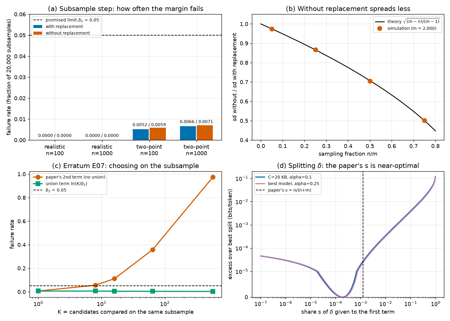
Panel (b) uses a small population (\(m = 2{,}000\), two-point) so that the sampling fraction \(n/m\) is not tiny. The ratio of spreads, without replacement over with, is 0.975, 0.867, 0.705 and 0.501 for \(n = 100\), 500, 1,000 and 1,500, matching the finite-population correction \(\sqrt{(m-n)/(m-1)}\) = 0.975, 0.866, 0.707 and 0.500 of Chapter 1. At the paper's \(n/m = 0.001247\) the correction is invisible, so the two schemes give the same numbers in practice.

(e) End-to-end coverage of Eq. (3)

Section [6] simulates the whole pipeline in a toy world where the true risks are known. There are 20 hypotheses with true risks spread evenly from 0.40 to 0.50 and a prior that halves from one hypothesis to the next. Each document's loss is 0 or 1 (\(\Delta = 1\)). In each of 5,000 runs: draw \(m = 1{,}000\) documents, train by choosing the hypothesis that minimizes training risk plus its complexity term, then draw \(n = 100\) documents with replacement and compute Eq. (3).

bound	failure rate (limit 0.05)
Eq. (3), as derived	0.0004
Eq. (1) with the full \(\hat R\) (reference)	0.0044
Eq. (1) with \(\hat{\hat R}\) plugged in, no second term	0.2612

The last row is the mistake the second term prevents: substituting the cheap estimate into Eq. (1) without paying makes the "95 % guarantee" fail about a quarter of the time.

(f) Choosing on the subsample (erratum E07)

Section [7] isolates the second stage. It fixes a training set of \(m = 20{,}000\) documents and 576 candidate hypotheses whose per-document losses are 0 or 1 at random, so every candidate has training risk close to 0.5. In each of 5,000 runs it draws \(n = 100\) documents, picks the candidate with the lowest subsampled risk among the first \(K\), and checks the second-stage claim with \(\delta_2 = 0.05\).

\(K\)	paper's margin 0.1224 fails	union margin fails	union margin
1	0.0062	0.0062	0.1224
8	0.0556	0.0062	0.1593
16	0.1110	0.0046	0.1698
64	0.3574	0.0038	0.1891
576	0.9748	0.0028	0.2162

With 576 candidates, the paper's second term is wrong almost every time in this toy world; the union-corrected term never exceeds its 0.05 budget. These candidates are independent of one another, which is the worst case. The paper's candidates (the same weights with different α, or models with different \(d\)) are strongly correlated, so the real over-optimism is much smaller than the union price, as Chapter 10's near-copies experiment showed. But only the corrected term is a theorem.

For the paper's best model the correction costs +0.0635 (\(N_{\text{sel}} = 8\)), +0.1082 (48) or +0.1614 (576) bits per token (section [7]); see the E07 box above.

(g) The δ split: the paper's s versus the true optimum

PAPER §A.3, p. 14 The paper picks \(\delta_1 = s\delta\), \(\delta_2 = (1-s)\delta\) with \(s = n/(n+m)\) as the solution of an optimization.

Paper erratum E06: s = n/(n+m) optimizes a proxy, not the bound

PAPER §A.3, p. 14 The split is derived by minimizing the single root \(\sqrt{\ln(1/\delta_1)/(2m) + \ln(1/\delta_2)/(2n)}\) with \(\delta_1+\delta_2=\delta\).

MY EXPLANATION The bound actually used is a sum of two roots, and its first root also contains \(\ln\frac1{P(h)}\). The proxy's minimizer is not the bound's minimizer. Any split with \(\delta_1+\delta_2=\delta\) gives a valid bound, so validity is unaffected; the only question is how much tightness is lost. Section [8]:

setting	true optimum \(s^*\)	paper's \(s\)	gain from \(s^*\) (bits/token)
\(C\) = 20 KB, \(\alpha = 0.1\)	\(1.814\times10^{-4}\)	\(1.247\times10^{-3}\)	0.000027
best model, \(\alpha = 0.25\)	\(1.995\times10^{-4}\)	\(1.247\times10^{-3}\)	0.000024
no complexity (\(\ln\frac1{P}=0\)), \(\alpha = 0.25\)	\(2.306\times10^{-2}\)	\(1.247\times10^{-3}\)	0.001421

The true optimum gives the first stage 6.87 and 6.25 times less failure budget than the paper does (first two rows; section [8]), but the gain is tens of millionths of a bit per token. Panel (d) of the figure shows why: the sum depends on the split only through logarithms, so it is very flat (erratum E06).

(h) The speed-up claims

PAPER §1, p. 1 The introduction says subsampling makes bound computation "900 times faster". PAPER §1, p. 2 The contributions list says the evaluation takes 45 minutes on a single GPU instead of 3 days on 8 GPUs.

Paper erratum E19: 900× does not follow from the stated times

MY EXPLANATION Section [9]: 3 days × 24 hours × 8 GPUs = 576 GPU-hours, against 45 minutes × 1 GPU = 0.75 GPU-hours. That is a factor of 768 in GPU time, or 72 / 0.75 = 96 in wall-clock time. The ratio of documents is \(m/n = 800.98\). None of these is 900. The order of magnitude (hundreds) is right; the exact figure is not supported by anything in the paper (erratum E19).

Paper erratum E20: '10's of millions' of documents

PAPER §4.4, p. 6 The text speaks of "dataset sizes in the 10's of millions". MY EXPLANATION OpenWebText has 8,009,762 training documents [SOURCE: nanoGPT prepare.py], under ten million. With 9,035,582,198 tokens, a document averages 1,128.1 tokens, so the 10,000 subsampled documents hold about 11.28 million tokens (section [9]). No number in the bound changes (erratum E20).

Going deeper

Everything in this section is MY EXPLANATION unless tagged.

The five blocks below give the full proof of Eq. (3), the δ-split calculus, the proof that sampling without replacement is safe, the formal repair for selection on the subsample, and the edge cases.

Going deeper: full proof of Eq. (3) / Eq. (8)

Setting. \(\mathcal H\) is a finite (or countable) set of hypotheses with prior \(P\), fixed before any data. The training set \(X = (X_1,\dots,X_m)\) has i.i.d. documents. Training is any rule \(\hat h = \hat h(X)\) (it may use extra randomness of its own; include that randomness in "\(X\)" below). For every \(h\), the per-document loss \(R(h, x)\) lies in an interval \([a_h, a_h + \Delta]\) fixed before the data (for smoothed bits per token, \([\log_2(V/\alpha) - \Delta(\alpha), \log_2(V/\alpha)]\), which depends on the α inside \(h\) but not on the data).

The subsample \(\sigma = (\sigma(1), \dots, \sigma(n))\) has i.i.d. entries, each uniform on \(\{1, \dots, m\}\), and \(\sigma\) is independent of \(X\) (requirements (i) and (ii)). \(\hat h\) is a function of \(X\) only (requirement (iii)).

The two bad events. Fix \(\delta_1, \delta_2 > 0\) with \(\delta_1 + \delta_2 = \delta\). Define

\[ E_1 = \Big\{\exists h \in \mathcal H:\ R(h) > \hat R(h) + \Delta\sqrt{\tfrac{\ln(1/P(h)) + \ln(1/\delta_1)}{2m}}\Big\}, \]

\[ E_2 = \Big\{\hat R(\hat h) > \hat{\hat R}(\hat h) + \Delta\sqrt{\tfrac{\ln(1/\delta_2)}{2n}}\Big\}. \]

\(E_1\) depends on \(X\) only. \(E_2\) depends on \(X\) (through \(\hat h\) and \(\hat R\)) and on \(\sigma\).

Step 1: \(\Pr[E_1] \le \delta_1\). This is Theorem A.1 (Chapter 11) with \(\delta_1\) in place of \(\delta\). The probability is over the draw of \(X\). Because \(E_1\) is a statement about all \(h\) at once, its complement covers \(\hat h\) whatever rule produced it.

Step 2: \(\Pr[E_2 \mid X = x] \le \delta_2\) for every possible training set \(x\). Fix \(x = (x_1,\dots,x_m)\). Then \(g = \hat h(x)\) is one fixed hypothesis, and the list \(\ell_j = R(g, x_j)\), \(j = 1,\dots,m\), is a fixed list of \(m\) numbers in \([a_g, a_g+\Delta]\). Define \(Z_i = \ell_{\sigma(i)}\) for \(i = 1, \dots, n\).

• Because \(\sigma\) is independent of \(X\), conditioning on \(X = x\) does not change the distribution of \(\sigma\): its entries are still i.i.d. uniform on \(\{1,\dots,m\}\).
• So \(Z_1, \dots, Z_n\) are i.i.d. given \(X = x\), each in an interval of width \(\Delta\).
• Their common conditional expectation is \(\mathbb E[Z_i \mid X = x] = \sum_{j=1}^m \frac1m \ell_j = \hat R(g)\).
• Their average is \(\frac1n\sum_i Z_i = \hat{\hat R}(g)\).

Apply Hoeffding's inequality in mean form, lower tail (Chapter 9), to the conditional distribution: for \(t > 0\),

\[ \Pr\Big[\hat{\hat R}(g) \le \hat R(g) - t \,\Big|\, X = x\Big] \le \exp\Big(-\frac{2nt^2}{\Delta^2}\Big). \]

Choose \(t = \Delta\sqrt{\ln(1/\delta_2)/(2n)}\). Then \(2nt^2/\Delta^2 = 2n\cdot\Delta^2\ln(1/\delta_2)/(2n)/\Delta^2 = \ln(1/\delta_2)\), and the right side is \(e^{-\ln(1/\delta_2)} = \delta_2\). The event \(E_2\) given \(X = x\) is \(\{\hat R(g) > \hat{\hat R}(g) + t\}\), that is \(\{\hat{\hat R}(g) < \hat R(g) - t\}\), which is contained in the event with "\(\le\)". So \(\Pr[E_2 \mid X = x] \le \delta_2\). Here the probability is over \(\sigma\) alone; \(x\), \(g\) and the list \(\ell\) are fixed.

Step 2, continued: remove the conditioning. A document is a finite sequence of tokens, so \(X\) takes countably many values. By the law of total probability (Chapter 1),

\[ \Pr[E_2] = \sum_x \Pr[X = x]\,\Pr[E_2 \mid X = x] \le \sum_x \Pr[X = x]\,\delta_2 = \delta_2 . \]

Now the probability is over both \(X\) and \(\sigma\). (If training uses its own random seed, sum over seeds as well; nothing changes.)

Step 3: union and chaining. By the union bound (Chapter 10), \(\Pr[E_1 \cup E_2] \le \delta_1 + \delta_2 = \delta\). So with probability at least \(1-\delta\) neither happens. Then, from "not \(E_1\)" applied to \(h = \hat h\), and then "not \(E_2\)",

\[ \begin{aligned} R(\hat h) &\le \hat R(\hat h) + \Delta\sqrt{\frac{\ln\frac{1}{P(\hat h)} + \ln\frac{1}{\delta_1}}{2m}} \\ &\le \hat{\hat R}(\hat h) + \Delta\sqrt{\frac{\ln\frac{1}{P(\hat h)} + \ln\frac{1}{\delta_1}}{2m}} + \Delta\sqrt{\frac{\ln\frac{1}{\delta_2}}{2n}} . \end{aligned} \]

Substituting \(\delta_1 = s\delta\) and \(\delta_2 = (1-s)\delta\) gives Eq. (8), which is Eq. (3). \(\square\)

Where each requirement was used. (i) independence of \(\sigma\) and \(X\): so that conditioning on \(X\) leaves \(\sigma\) uniform. (ii) uniform sampling: so that \(\mathbb E[Z_i \mid X = x] = \hat R(g)\); a sampling scheme that favours some documents (short ones, say) would centre the subsample on a different number. (iii) \(\hat h\) a function of \(X\) only: so that \(g\) is fixed when \(X\) is fixed; if \(\hat h\) depends on \(\sigma\), the list \(\ell\) changes with \(\sigma\) and the \(Z_i\) are not draws from a fixed list.

Units. \(R\), \(\hat R\), \(\hat{\hat R}\), \(\Delta\) and \(t\) are in loss units (bits per token, or a fraction). \(\ln(1/P)\) and \(\ln(1/\delta_i)\) are in nats. \(nt^2/\Delta^2\) is a pure number, as an exponent must be.

Going deeper: the δ split, the proxy and the true optimum

The proxy (the paper's derivation, made explicit). Minimize \(\sqrt{\ln(1/\delta_1)/(2m) + \ln(1/\delta_2)/(2n)}\) subject to \(\delta_1 + \delta_2 = \delta\). The square root is increasing, so it suffices to minimize the inside. Substitute \(\delta_2 = \delta - \delta_1\), for \(0 < \delta_1 < \delta\):

\[ g(\delta_1) = \frac{\ln(1/\delta_1)}{2m} + \frac{\ln(1/(\delta-\delta_1))}{2n} = -\frac{\ln\delta_1}{2m} - \frac{\ln(\delta-\delta_1)}{2n}. \]

Differentiate (the derivative of \(\ln u\) is \(1/u\); the inner derivative of \(\delta - \delta_1\) is \(-1\)):

\[ g'(\delta_1) = -\frac{1}{2m\delta_1} + \frac{1}{2n(\delta - \delta_1)} . \]

Set it to zero: \(2n(\delta - \delta_1) = 2m\delta_1\), so \(\delta_1(m + n) = n\delta\) and \(\delta_1 = \frac{n}{n+m}\delta = s\delta\). The second derivative, \(g''(\delta_1) = \frac{1}{2m\delta_1^2} + \frac{1}{2n(\delta-\delta_1)^2}\), is positive, so \(g\) is convex and this is its unique minimum. Section [8] confirms it numerically (\(s = 0.001247\) both ways).

The true objective. The bound depends on the split through

\[ F(\delta_1) = \Delta\left[\sqrt{\frac{L + \ln(1/\delta_1)}{2m}} + \sqrt{\frac{\ln(1/(\delta-\delta_1))}{2n}}\right], \qquad L = \ln\frac{1}{P(h)} . \]

Write \(T_1 = \sqrt{(L + \ln(1/\delta_1))/(2m)}\) and \(T_2 = \sqrt{\ln(1/\delta_2)/(2n)}\). By the chain rule, the derivative of \(\sqrt{u}\) is \(1/(2\sqrt u)\), and \(u = (L + \ln(1/\delta_1))/(2m)\) has derivative \(-1/(2m\delta_1)\), so

\[ \frac{F'(\delta_1)}{\Delta} = -\frac{1}{4m\delta_1 T_1} + \frac{1}{4n\delta_2 T_2} . \]

Setting this to zero gives the optimality condition

\[ \frac{\delta_1}{\delta_2} = \frac{n}{m}\cdot\frac{T_2}{T_1} . \]

Compare the proxy's \(\delta_1/\delta_2 = n/m\). The true optimum multiplies it by \(T_2/T_1\), the ratio of the two margins (without \(\Delta\)). For the best model, at the optimum, \(T_2/T_1 = 0.160\) (section [8]), which is why \(s^*\) is \(s/s^* = 6.25\) times smaller than \(s\). The condition is implicit (\(T_1\) and \(T_2\) depend on \(\delta_1\)), so the script solves it numerically and then checks it: \(\delta_1/\delta_2\) and \(nT_2/(mT_1)\) agree to five digits in every row of section [8]. With no complexity (\(L = 0\)) the first margin is small, \(T_2/T_1\) is large, and \(s^*\) moves above \(s\) (\(2.306\times10^{-2}\)).

Why the gain is tiny. Near the optimum, \(F\) changes only to second order. And the split enters only through \(\ln(1/\delta_i)\): shrinking \(\delta_1\) by the factor 6.25 adds \(\ln 6.25 = 1.83\) nats (section [8]) to a numerator of about 93,900 nats.

Going deeper: sampling without replacement is safe (Hoeffding 1963, Theorem 4), with proof

Statement. SOURCE: Hoeffding 1963, Theorem 4 Let \(a_1, \dots, a_N\) be numbers (the population) and \(n \le N\). Let \(S_{\text{w}} = \sum_{r=1}^n a_{I_r}\) with \(I_1, \dots, I_n\) i.i.d. uniform on \(\{1,\dots,N\}\) (with replacement), and \(S_{\text{o}} = \sum_{r=1}^n a_{J_r}\) with \((J_1, \dots, J_n)\) a uniformly random ordered sample of \(n\) distinct indices (without replacement). Then for every convex function \(f\), \(\mathbb E f(S_{\text{o}}) \le \mathbb E f(S_{\text{w}})\). (Hoeffding states it for continuous convex \(f\); with finitely many values, as here, convexity is enough.)

MY EXPLANATION The proof below is a coupling: we build \(S_{\text{w}}\) and a copy of \(S_{\text{o}}\) on the same random experiment so that \(S_{\text{o}}\) is the conditional average of \(S_{\text{w}}\), then apply Jensen.

Step 1: split a with-replacement sequence into "pattern" and "identities". Take a sequence \(i = (i_1,\dots,i_n)\). List its distinct values in order of first appearance, \(j_1, \dots, j_k\); \(k\) is the number of distinct values. Its pattern \(\pi\) records, for each position \(r\), which of the \(k\) distinct values sits there. Example with \(n = 4\): \((7, 3, 7, 9)\) has \(k = 3\), identities \((7, 3, 9)\) and pattern \((1, 2, 1, 3)\).

The map \(i \mapsto (\pi, (j_1,\dots,j_k))\) is a one-to-one correspondence between sequences and pairs (a pattern with \(k\) blocks, an ordered \(k\)-tuple of distinct indices): every such pair rebuilds exactly one sequence. Each sequence has probability \(N^{-n}\). Hence, for a pattern \(\pi\) with \(k\) blocks and any ordered \(k\)-tuple of distinct indices,

\[ \Pr\big[\text{pattern} = \pi,\ (J_1,\dots,J_k) = (j_1,\dots,j_k)\big] = N^{-n} . \]

There are \(N(N-1)\cdots(N-k+1)\) such tuples, so \(\Pr[\text{pattern} = \pi] = N^{-n}N(N-1)\cdots(N-k+1)\), and given the pattern, every ordered \(k\)-tuple of distinct indices has the same conditional probability \(1/(N(N-1)\cdots(N-k+1))\). In words: given the pattern, the identities are a uniform without-replacement sample of size \(k\).

Let \(c_t\) be the number of positions in block \(t\) (the multiplicity of the \(t\)-th distinct value). It is a function of the pattern, \(c_t \ge 1\) and \(\sum_{t=1}^k c_t = n\). Grouping equal terms, \(S_{\text{w}} = \sum_{t=1}^{k} c_t\, a_{J_t}\).

Step 2: extend to \(n\) identities. Given the pattern and \(J_1,\dots,J_k\), draw \(J_{k+1},\dots,J_n\) uniformly without replacement from the \(N-k\) unused indices, using extra independent randomness, and set \(c_t = 0\) for \(t > k\). Then \(S_{\text{w}} = \sum_{t=1}^{n} c_t a_{J_t}\) still holds (the new terms have weight 0). Given the pattern, each ordered \(n\)-tuple of distinct indices now has probability \(\frac{1}{N\cdots(N-k+1)}\cdot\frac{1}{(N-k)\cdots(N-n+1)} = \frac{(N-n)!}{N!}\), the same for all tuples. So \(J = (J_1,\dots,J_n)\) is a uniform ordered without-replacement sample of size \(n\), whatever the pattern: \(J\) is independent of the pattern, hence of the weights \(c = (c_1, \dots, c_n)\). The weights satisfy \(c_t \ge 0\) and \(\sum_t c_t = n\).

Step 3: average over the order. Let \(A = \{J_1, \dots, J_n\}\) be the unordered set. Given \(A\) and \(c\), each of the \(n!\) orderings of \(A\) is equally likely (each has probability \((N-n)!/N!\) before conditioning, and \(J\) is independent of \(c\)). In a uniformly random ordering, each element of \(A\) is equally likely to sit in slot \(t\): \((n-1)!\) of the \(n!\) orderings put a given element there. So \(\mathbb E[a_{J_t} \mid A, c] = \frac1n\sum_{j \in A} a_j\) for every \(t\), and by linearity

\[ \mathbb E[S_{\text{w}} \mid A, c] = \sum_{t=1}^n c_t \cdot \frac1n\sum_{j\in A} a_j = \frac{\sum_t c_t}{n}\sum_{j\in A} a_j = \sum_{j\in A} a_j . \]

Step 4: Jensen given \((A, c)\). Given \((A, c)\), \(S_{\text{w}}\) is a random variable taking finitely many values (one per ordering). Jensen's inequality (Chapter 9) applied to this conditional distribution gives

\[ \mathbb E[f(S_{\text{w}}) \mid A, c] \ge f\big(\mathbb E[S_{\text{w}} \mid A, c]\big) = f\Big(\sum_{j\in A} a_j\Big). \]

Step 5: average over \((A, c)\). By the tower rule (Chapter 1), \(\mathbb E f(S_{\text{w}}) = \mathbb E\big[\mathbb E[f(S_{\text{w}}) \mid A, c]\big] \ge \mathbb E f\big(\sum_{j\in A} a_j\big)\). Since \(A\) is the set of a uniform without-replacement sample, \(\sum_{j\in A} a_j\) has exactly the distribution of \(S_{\text{o}}\). Hence \(\mathbb E f(S_{\text{o}}) \le \mathbb E f(S_{\text{w}})\). \(\square\)

Step 6: Hoeffding without replacement. Let \(\mu = \frac1N\sum_j a_j\) (in our use, \(\mu = \hat R(g)\) and \(N = m\)), with every \(a_j\) in an interval of width \(\Delta\). Both sums have mean \(n\mu\). Fix \(\lambda > 0\). The function \(x \mapsto e^{-\lambda(x - n\mu)}\) is convex, so by the Chernoff method and Steps 1–5,

\[ \begin{aligned} \Pr[S_{\text{o}} - n\mu \le -\varepsilon] &\le e^{-\lambda\varepsilon}\,\mathbb E\,e^{-\lambda(S_{\text{o}} - n\mu)} \\ &\le e^{-\lambda\varepsilon}\,\mathbb E\,e^{-\lambda(S_{\text{w}} - n\mu)} \le \exp\Big(-\lambda\varepsilon + \frac{\lambda^2 n\Delta^2}{8}\Big), \end{aligned} \]

where the last step is Chapter 9's proof for independent terms (factorize, then Hoeffding's lemma). Optimizing \(\lambda\) exactly as in Chapter 9 gives \(\exp(-2\varepsilon^2/(n\Delta^2))\); with \(\varepsilon = nt\) it is \(\exp(-2nt^2/\Delta^2)\), the same limit. So Step 2 of the Eq. (3) proof goes through unchanged for sampling without replacement (requires \(n \le m\)).

Exact check (section [5]). Population \((0, 1, 1, 2, 5, 9)\), samples of size 3, all \(6^3 = 216\) with-replacement sequences and all 120 without-replacement sequences enumerated:

\(f\)	\(\mathbb E f\), with	\(\mathbb E f\), without
\(e^{0.5(S - n\mu)}\)	66.9996	5.2887
\(e^{-0.5(S - n\mu)}\)	7.9693	5.2887
\((S - n\mu)^2\)	29.0000	17.4000
\(\lvert S - 10\rvert\)	4.5093	3.6000

(The two exponentials have the same value without replacement because here the complement of a 3-element sample is another 3-element sample with sum \(18 - S\), so \(S - 9\) is symmetric.) The third row is the variance: \(17.4 = 29 \times (6-3)/(6-1)\), Chapter 1's finite-population correction.

What the theorem does not say. It compares expectations of convex functions, not tail probabilities. The tail itself can come out slightly larger without replacement at a given threshold; section [4] shows 0.0059 against 0.0052, within simulation noise. What is guaranteed is that the same Hoeffding limit holds for both.

Going deeper: repairing selection on the subsample (erratum E07)

The rigorous version. Suppose that after training, the training set \(X\) (and training's own randomness) determines a list of candidates \(h_1(X), \dots, h_N(X)\), each with its own width \(\Delta_k\). For example, the trained weights with each of the 8 values of α, or the trained models for each \(d\). Then \(\sigma\) is drawn, all candidates are evaluated on it, and any rule, looking at anything, picks the reported \(\hat h\) among them. Define

\[ E_2' = \Big\{\exists k \le N:\ \hat R(h_k) > \hat{\hat R}(h_k) + \Delta_k\sqrt{\tfrac{\ln(N/\delta_2)}{2n}}\Big\}. \]

Fix \(X = x\). Each \(h_k(x)\) is fixed, so Step 2 of the main proof at level \(\delta_2/N\) gives probability at most \(\delta_2/N\) for each \(k\), and the union bound over \(k\) gives \(\Pr[E_2' \mid X = x] \le N\cdot\delta_2/N = \delta_2\). Remove the conditioning as before. Outside \(E_2'\) the inequality holds for every candidate, so also for the one picked. The first stage needs no change: \(E_1\) already covers all hypotheses, and the hyperparameter bits in \(\ln\frac1{P(h)}\) pay for the choice there (Chapter 14). The result is Eq. (3) with \(\ln\frac{N}{(1-s)\delta}\) in the second term.

What \(N\) is in the paper. §6.1 optimizes α for each model on the subsample (8 values); App. C reports the lowest bound over \(r\), \(d\), quantization levels and α. If all of these were compared on one subsample, \(N = 576\) (the full grid; Chapter 24). If only α and \(d\), \(N = 48\). If each model had its own subsample but α was chosen on it, \(N = 8\). The paper does not say whether the same \(\sigma\) was reused, so we report all three.

A cheaper repair. Use two independent subsamples: choose the candidate on the first, then compute the reported bound on a fresh second subsample. Given \(X\) and the first subsample, the chosen model is fixed, so the second subsample's Hoeffding step is valid with \(N = 1\). The cost is one more evaluation of 10,000 documents, and \(\delta\) is unchanged.

Why the toy numbers overstate the real effect. In section [7] the candidates' per-document losses are independent, so some candidate is almost always lucky. The paper's candidates share most of their behaviour: the same model smoothed with α = 0.1 or 0.25 makes the same mistakes on the same documents. Their luck is shared, as in Chapter 10's near-copies experiment, and the selection effect is much smaller than the union price. The union price is what a proof can promise without further assumptions.

Going deeper: edge cases and fine print

• One-sided. Eq. (3) is an upper bound on \(R(\hat h)\). Only the lower tail of \(\hat{\hat R}\) matters (an underestimate of \(\hat R\)), so the one-sided Hoeffding limit \(\delta_2\) is used, not \(2\delta_2\).
• Documents, not tokens. \(\sigma\) samples documents uniformly. Long and short documents count equally, matching the definition of \(\hat R\) as an average of per-document losses (Chapter 15). Sampling tokens uniformly would centre the estimate on a token-weighted average, a different quantity.
• \(n > m\). With replacement, any \(n\) is allowed (and \(s = n/(n+m)\) is still in \((0,1)\)). Without replacement, \(n \le m\), and at \(n = m\) the subsample is the whole training set: \(\hat{\hat R} = \hat R\) exactly, and the second term is pure waste.
• Training on part of the data. PAPER §4.4, p. 6 The paper notes that the model need not be trained on the entire training set. MY EXPLANATION Correct: Theorem A.1 holds for every hypothesis, however chosen. But the subsample must be drawn from all \(m\) documents that enter \(\hat R\) and the \(m\) in the first term, not only from the documents used in training.
• The subsample must come after training, or at least not feed into it. If the same 10,000 documents were used for early stopping or for choosing the learning rate, \(\hat h\) would depend on \(\sigma\), and requirement (iii) would fail. PAPER §4.4, p. 6 The paper evaluates the subsample after the model has been trained.
• The interval must not depend on \(\sigma\). For smoothed bits per token the window is fixed by α. If α is chosen on the subsample, both the hypothesis and its window depend on \(\sigma\): that is erratum E07 again.
• Reusing one subsample for many reported bounds. Each bound, read alone, holds with probability at least \(1-\delta\) if its model was fixed before \(\sigma\). A claim that all reported bounds hold at once needs a union over them.
• Code check. [SOURCE: authors' code, llm_subsampling_bound] The authors' function computes sqrt((div - log(r*eps))/(2*data_size)) + sqrt(-log((1-r)*eps)/(2*sample_size)) with r = sample_size/(sample_size+data_size), multiplied by the interval width: exactly Eq. (8) with natural logs. Their document sampler draws indices with np.random.randint, that is, with replacement.

Common misconceptions

Everything in this section is MY EXPLANATION.

• Misconception: The subsampling bound is a statement about the 10,000 subsampled documents. — Actually: It bounds \(R(\hat h)\), the expected loss on a fresh document from the population. The subsample is only a cheap way to estimate \(\hat R(\hat h)\), and the second term pays for the estimation error.
• Misconception: Since the 10,000 documents are random documents from the population, one could apply Eq. (1) with \(n\) in place of \(m\) and skip the two stages. — Actually: That is valid (for sampling without replacement) but useless: the complexity term would be divided by \(n\) instead of \(m\), giving 47.8683 bits per token for the best model. The two-stage argument pays for complexity with \(m\) and only for estimation with \(n\).
• Misconception: The second term is negligible. — Actually: For the best model it is 0.2106 bits per token, 0.160 times the complexity term and 6.03 % of the margin to the random-guess level. For top-k error it is 1.2 percentage points.
• Misconception: The hyperparameter bits in \(\ln\frac1{P(h)}\) pay for choosing α on the subsample. — Actually: They pay in the first term only. The second term is a single-hypothesis bound; comparing candidates on the same subsample needs \(\ln N_{\text{sel}}\) added inside it (erratum E07).
• Misconception: Sampling without replacement always fails less often than with replacement. — Actually: Hoeffding's Theorem 4 compares expectations of convex functions (it is why the same limit holds), not the tail probabilities themselves. At the paper's \(n/m = 0.001247\) the two schemes are practically identical.
• Misconception: \(s = n/(n+m)\) is the optimal way to split \(\delta\). — Actually: It optimizes a proxy. The true optimum gives the first stage 6.25 times less (best model), but improves the bound by only 0.000024 bits per token (erratum E06).

Self-test

Q1. For the paper's best model (\(\Delta(0.25) = 17.2020\) bits per token, \(\hat{\hat R} = 10.5945\)), the second term is 0.2106 at \(n = 10{,}000\). What is it at \(n = 1{,}000\), roughly why, and what would the bound become if the subsampled risk were unchanged? How many documents would bring the second term down to 0.05 bits per token?

Answer

The second term is \(\Delta\sqrt{\ln(1/((1-s)\delta))/(2n)}\). Dividing \(n\) by 10 multiplies it by \(\sqrt{10}\), apart from a negligible change in \(s\): the script prints 0.6658 bits per token. The bound becomes 12.5774 instead of 12.1222 (script section [3]). Solving \(\Delta\sqrt{\ln(1/\delta_2)/(2n)} = 0.05\) for \(n\) gives \(n = \Delta^2\ln(1/\delta_2)/(2\cdot0.05^2)\) = 177,367 documents.

Q2. An engineer draws one subsample of 10,000 documents, evaluates the trained model smoothed with each of the 8 values of α on it, reports the α with the lowest Eq. (3) bound, and pays \(\log_2 8 = 3\) hyperparameter bits in \(\ln\frac1{P(h)}\). Is the reported number covered by the theorem? If not, give two ways to fix it.

Answer

No. The 3 bits repair the first term, which is a union over all hypotheses. The second term is a Hoeffding bound for one hypothesis fixed before \(\sigma\) was drawn; the reported α was chosen using \(\sigma\), so requirement (iii) fails. Fix 1: replace \(\ln\frac1{(1-s)\delta}\) by \(\ln\frac{8}{(1-s)\delta}\) (a union over the 8 candidates, which are fixed by the training set); for the best model this gives 12.1857 instead of 12.1222. Fix 2: choose α on one subsample and compute the reported bound on a second, independent subsample.

Q3. In the proof of Eq. (3), the trained model \(\hat h\) depends on all \(m\) training documents, including the ones the subsample picks. Why is the Hoeffding step over \(\sigma\) still valid? Give one change to the procedure that would break it.

Answer

The step is made with the training set held fixed. Given \(X = x\), the model \(\hat h(x)\) is one fixed function and its per-document losses form a fixed list of \(m\) numbers. The subsample, drawn with randomness independent of \(X\), picks \(n\) entries of that list uniformly at random, so they are i.i.d. with mean \(\hat R(\hat h(x))\), and Hoeffding applies. The conditional limit \(\delta_2\) holds for every \(x\), so it also holds on average over \(X\) (law of total probability). It breaks if \(\sigma\) depends on \(X\) (for example, sampling only short documents, which changes the mean), or if \(\hat h\) depends on \(\sigma\) (for example, using the subsample for early stopping or to pick α).

Code for this chapter

Run it from the project root:

.venv/Scripts/python explainer/code/ch17_subsampling.py

Source: ch17_subsampling.py

"""Chapter 17 - the subsampling bound, Eq. (3) / Eq. (8) of arXiv 2312.17173.

Reproduces / checks:
  [1] the delta split s = n/(n+m) and the logs it creates (delta, m from SOURCE: authors' code, nanoGPT);
  [2] Table 1's 12.12 bits/token from the Fig. 2 best model (alpha=0.25, Rhathat=10.5945, C=16.5325 KB),
      and the price of subsampling for that model;
  [3] the size of the second (subsample) term for several Delta and n;
  [4] coverage of the subsample step (Hoeffding over sigma, training set fixed), with and without replacement;
  [5] exact check of Hoeffding (1963) Theorem 4: E f(sum without repl.) <= E f(sum with repl.) for convex f;
  [6] end-to-end coverage of Eq. (3) in a toy world;
  [7] erratum E07: choosing among K candidates on the subsample breaks the second term; the union repair;
  [8] the delta split: proxy optimum s = n/(n+m) vs the true optimum of the sum of square roots (erratum E06);
  [9] the speed-up arithmetic of Section 1 (erratum E19) and dataset size (erratum E20).
Figure: docs/assets/fig/ch17_coverage.png
"""
from __future__ import annotations

import itertools
import json
import math
import sys
from pathlib import Path

import numpy as np
from scipy.optimize import minimize_scalar

HERE = Path(__file__).resolve().parent
sys.path.insert(0, str(HERE))
import pacbound as pb  # noqa: E402

import matplotlib  # noqa: E402
matplotlib.use("Agg")
import matplotlib.pyplot as plt  # noqa: E402

OUT_TXT = HERE / "outputs" / "ch17_subsampling.txt"
OUT_FIG = HERE.parent / "docs" / "assets" / "fig" / "ch17_coverage.png"
lines: list[str] = []


def out(s: str = "") -> None:
    print(s)
    lines.append(s)


m, n, delta = pb.M_DOCS, pb.N_SUB, pb.DELTA
s = n / (n + m)

# ---------------------------------------------------------------------------
out("[1] The delta split (delta=0.05, m=8,009,762 [SOURCE: authors' code / nanoGPT]; n=10,000 [PAPER])")
d1, d2 = s * delta, (1 - s) * delta
out(f"    s = n/(n+m) = {s:.6f};  delta1 = s*delta = {d1:.4e};  delta2 = (1-s)*delta = {d2:.6f}")
out(f"    ln(1/delta) = {math.log(1/delta):.4f} nats;  ln(1/(s delta)) = {math.log(1/d1):.4f} nats "
    f"(+{math.log(1/d1)-math.log(1/delta):.4f});  ln(1/((1-s)delta)) = {math.log(1/d2):.6f} nats")

# ---------------------------------------------------------------------------
out("[2] Best GPT-2-small model (Fig. 2 / errata F): alpha=0.25, Rhathat=10.5945 bits/token, C=16.5325 KB")
alpha = 0.25
_, _, Dlt = pb.smoothing_interval(alpha)
# exact values read from the PDF's vector data by fig_extract.py (same source as ch14_budget.py)
_fig = json.loads((HERE / "outputs" / "fig_extract.json").read_text(encoding="utf-8"))["figure2"]["left"]
_i = min(range(len(_fig["bound"])), key=lambda i: _fig["bound"][i]["value"])
C_bits = _fig["compressed_size_kb"][_i]["value"] * 8192    # 1 KB = 8192 bits (erratum E35)
price = pb.log_inv_prior_nats_from_bits(C_bits)
R2 = _fig["empirical_risk"][_i]["value"]
out(f"    (exact figure read: C = {C_bits/8192:.4f} KB, Rhathat = {R2:.4f} bits/token)")
t1, t2 = pb.eq3_terms(price, m, n, delta, Dlt)
b = pb.eq3_bound(R2, price, m, n, delta, Dlt)
out(f"    Delta(0.25) = {Dlt:.4f} bits/token; C = {C_bits:,.2f} bits; ln 1/P(h) = {price:,.2f} nats "
    f"(C ln2 alone = {C_bits*pb.LN2:,.2f})")
out(f"    first term = {t1:.5f}, second term = {t2:.5f}, bound = {b:.4f} bits/token  (paper Table 1: 12.12, "
    f"diff {b-12.12:+.4f})")
assert abs(b - 12.12) < 0.005
t1_full = pb.eq1_complexity(price, m, delta, Dlt)
out(f"    same model if Rhat were computed on all m docs (Eq. 1): term = {t1_full:.5f}; price of subsampling = "
    f"{t1 - t1_full:.6f} (first term) + {t2:.5f} (second) = {t1 - t1_full + t2:.4f} bits/token")
out(f"    second/first term = {t2/t1:.3f}; with the printed sum (no 1/n, erratum E03) Rhathat would be ~{R2*n:,.0f}")
t_alt = pb.eq1_complexity(price, n, delta, Dlt)
out(f"    alternative: Theorem A.1 on the n subsampled docs alone: term = {t_alt:.4f}, bound = {R2 + t_alt:.4f} "
    f"bits/token (vacuous: > {pb.random_guess_bpd():.3f})")
out(f"    as a share: {100*(t1-t1_full+t2)/b:.2f} % of the bound; {100*(t1-t1_full+t2)/(pb.random_guess_bpd()-b):.2f} "
    f"% of the gap to log2 V = {pb.random_guess_bpd():.3f}")

# ---------------------------------------------------------------------------
out("[3] Second term Delta*sqrt(ln(N_sel/((1-s)delta))/(2n)), n=10,000 (loss units)")
D01 = pb.smoothing_interval(0.1)[2]
out(f"    {'Delta':>18} | N_sel=1 | N_sel=8 | N_sel=48 | N_sel=576")
for name, D in [("1 (top-k, fraction)", 1.0), (f"{D01:.3f} (alpha=0.1)", D01), (f"{Dlt:.3f} (alpha=0.25)", Dlt)]:
    vals = [pb.eq3_terms(price, m, n, delta, D, n_selected=k)[1] for k in (1, 8, 48, 576)]
    out(f"    {name:>18} | " + " | ".join(f"{v:.4f}" for v in vals))
out("    second term vs n at Delta(0.25), N_sel=1:  " + ", ".join(
    f"n={k:,}: {pb.eq3_terms(price, m, k, delta, Dlt)[1]:.4f}" for k in (1_000, 10_000, 100_000, 1_000_000)))
out("    best-model bound (Eq. 3) vs n:  " + ", ".join(
    f"n={k:,}: {pb.eq3_bound(R2, price, m, k, delta, Dlt):.4f}" for k in (1_000, 10_000, 100_000)))
n_need = Dlt**2 * math.log(1 / d2) / (2 * 0.05**2)
out(f"    n needed for a second term of 0.05 bits/token at Delta(0.25): {n_need:,.0f} documents")

# ---------------------------------------------------------------------------
out("[4] Coverage of the subsample step: X fixed (m=100,000 doc losses in [0, 18.787]), sigma random, 20,000 draws")
rng = np.random.default_rng(0)
M_TOY, REPS, d2_toy, W = 100_000, 20_000, 0.05, D01
pops = {
    "realistic": np.clip(rng.lognormal(math.log(10.5), 0.12, M_TOY), 0, W),
    "two-point": W * (rng.random(M_TOY) < 0.5).astype(float),
}


def sample_wo(gen, N, k):
    """Uniform sample of k distinct indices from range(N): draw i.i.d. indices and keep first appearances
    (the sequence of first appearances of i.i.d. uniform draws is a uniform without-replacement sample)."""
    while True:
        draw = gen.integers(0, N, int(1.2 * k) + 50)
        _, first = np.unique(draw, return_index=True)
        if len(first) >= k:
            return draw[np.sort(first)[:k]]


out(f"    realistic population: mean {pops['realistic'].mean():.3f}, sd {pops['realistic'].std():.3f} bits/token "
    f"(ASSUMPTION, not from the paper)")
cov = {}
for pname, a in pops.items():
    mu = a.mean()
    for nn in (100, 1000):
        marg = W * math.sqrt(math.log(1 / d2_toy) / (2 * nn))
        res = {}
        for scheme in ("with", "without"):
            if scheme == "with":
                means = a[rng.integers(0, M_TOY, (REPS, nn))].mean(1)
            else:
                means = np.array([a[sample_wo(rng, M_TOY, nn)].mean() for _ in range(REPS)])
            fail = np.mean(mu > means + marg)
            res[scheme] = (fail, means.std())
            cov[(pname, nn, scheme)] = fail
        out(f"    {pname:9s} n={nn:5d}: margin {marg:.3f}; failure with={res['with'][0]:.4f}, "
            f"without={res['without'][0]:.4f} (limit {d2_toy}); sd with={res['with'][1]:.4f}, without={res['without'][1]:.4f}")
        assert res["with"][0] <= d2_toy and res["without"][0] <= d2_toy

out(f"    Monte Carlo standard error of a failure rate near 0.006 from 20,000 draws: {math.sqrt(0.006*0.994/REPS):.5f}")

# spread ratio on a small population, where n/m is not tiny
a_small = pops["two-point"][:2000]
mu_s = a_small.mean()
ratios = []
for nn in (100, 500, 1000, 1500):
    sw = a_small[rng.integers(0, 2000, (20000, nn))].mean(1)
    so = np.concatenate([a_small[np.argpartition(rng.random((2000, 2000)), nn, axis=1)[:, :nn]].mean(1)
                         for _ in range(10)])
    marg = W * math.sqrt(math.log(1 / d2_toy) / (2 * nn))
    ratios.append((nn / 2000, so.std() / sw.std(), math.sqrt((2000 - nn) / 1999)))
    out(f"    m=2,000 two-point, n={nn:5d}: sd ratio without/with = {so.std()/sw.std():.3f} "
        f"(theory sqrt((m-n)/(m-1)) = {math.sqrt((2000-nn)/1999):.3f}); failure with={np.mean(mu_s > sw + marg):.4f}, "
        f"without={np.mean(mu_s > so + marg):.4f}")

# ---------------------------------------------------------------------------
out("[5] Hoeffding 1963 Thm 4, exact enumeration: population (0,1,1,2,5,9), samples of size 3")
popE = np.array([0, 1, 1, 2, 5, 9], dtype=float)
NE, nE = len(popE), 3
S_with = np.array([popE[list(t)].sum() for t in itertools.product(range(NE), repeat=nE)])
S_wo = np.array([popE[list(t)].sum() for t in itertools.permutations(range(NE), nE)])
mE = nE * popE.mean()
fs = {"exp(0.5(S-n mu))": lambda x: np.exp(0.5 * (x - mE)), "exp(-0.5(S-n mu))": lambda x: np.exp(-0.5 * (x - mE)),
      "(S-n mu)^2": lambda x: (x - mE) ** 2, "|S-10|": lambda x: np.abs(x - 10)}
for nm, f in fs.items():
    ew, eo = f(S_with).mean(), f(S_wo).mean()
    out(f"    E f, f = {nm:18s}: with = {ew:9.4f}, without = {eo:9.4f}  (without <= with: {eo <= ew + 1e-12})")
    assert eo <= ew + 1e-12

# ---------------------------------------------------------------------------
out("[6] End-to-end coverage of Eq. (3), toy world: K=20 hypotheses, 0-1 doc losses (Delta=1), m=1,000, n=100")
K6, m6, n6, R6 = 20, 1000, 100, 5000
rng = np.random.default_rng(6)
p_true = np.linspace(0.40, 0.50, K6)                 # true risks R(h_k), known
prior = 0.5 ** np.arange(1, K6 + 1); prior /= prior.sum()
s6 = n6 / (n6 + m6)
lnP = np.log(1 / prior)
pen1 = np.sqrt((lnP + math.log(1 / (s6 * delta))) / (2 * m6))
pen2 = math.sqrt(math.log(1 / ((1 - s6) * delta)) / (2 * n6))
fail_eq3 = fail_no2 = fail_eq1 = 0
for r in range(R6):
    Xl = (rng.random((m6, K6)) < p_true).astype(np.float32)   # loss of h_k on doc j
    Rhat = Xl.mean(0)
    k = int(np.argmin(Rhat + pen1))                        # training: ERM with a prior (SRM)
    sig = rng.integers(0, m6, n6)                          # subsample, drawn after training
    Rhh = Xl[sig, k].mean()
    fail_eq3 += p_true[k] > Rhh + pen1[k] + pen2
    fail_no2 += p_true[k] > Rhh + math.sqrt((lnP[k] + math.log(1 / delta)) / (2 * m6))
    fail_eq1 += p_true[k] > Rhat[k] + math.sqrt((lnP[k] + math.log(1 / delta)) / (2 * m6))
out(f"    failure rate of Eq. (3): {fail_eq3/R6:.4f} (limit {delta}); Eq. (1) on full Rhat: {fail_eq1/R6:.4f}; "
    f"Eq. (1) with Rhathat plugged in (no 2nd term): {fail_no2/R6:.4f}")
assert fail_eq3 / R6 <= delta
e2e = (fail_eq3 / R6, fail_eq1 / R6, fail_no2 / R6)

# ---------------------------------------------------------------------------
out("[7] Erratum E07: pick the best of K candidates ON the subsample (X fixed, m=20,000, n=100, two-point 0/1)")
m7, n7, R7 = 20_000, 100, 5000
rng = np.random.default_rng(7)
L7 = (rng.random((m7, 576)) < 0.5).astype(np.int8)
Rhat7 = L7.mean(0)
sel = {}
for K in (1, 8, 16, 64, 576):
    fp = fu = 0
    mp = math.sqrt(math.log(1 / d2_toy) / (2 * n7))
    mu_ = math.sqrt(math.log(K / d2_toy) / (2 * n7))
    for r in range(R7):
        sig = rng.integers(0, m7, n7)
        sub = L7[sig, :K].mean(0)
        k = int(np.argmin(sub))
        fp += Rhat7[k] > sub[k] + mp
        fu += Rhat7[k] > sub[k] + mu_
    sel[K] = (fp / R7, fu / R7)
    out(f"    K={K:4d}: paper's term ({mp:.4f}) fails {fp/R7:.4f}; union term ({mu_:.4f}) fails {fu/R7:.4f} "
        f"(limit {d2_toy})")
    assert fu / R7 <= d2_toy
out(f"    best model with E07 repair (Delta(0.25)): N_sel=8 -> {pb.eq3_bound(R2, price, m, n, delta, Dlt, n_selected=8):.4f}, "
    f"48 -> {pb.eq3_bound(R2, price, m, n, delta, Dlt, n_selected=48):.4f}, "
    f"576 -> {pb.eq3_bound(R2, price, m, n, delta, Dlt, n_selected=576):.4f} bits/token (paper 12.12)")
out("    increase over 12.1222: " + ", ".join(f"N_sel={k}: +{pb.eq3_bound(R2, price, m, n, delta, Dlt, n_selected=k) - b:.4f}"
                                        for k in (8, 48, 576)))

# ---------------------------------------------------------------------------
out("[8] Delta split: proxy optimum s=n/(n+m) vs true optimum of the actual sum of square roots (erratum E06)")


def proxy(d1_):
    return math.sqrt(math.log(1 / d1_) / (2 * m) + math.log(1 / (delta - d1_)) / (2 * n))


def total(d1_, L, D):
    return D * (math.sqrt((L + math.log(1 / d1_)) / (2 * m)) + math.sqrt(math.log(1 / (delta - d1_)) / (2 * n)))


def argmin_log(fun):
    r = minimize_scalar(lambda u: fun(delta / (1 + math.exp(-u))), bounds=(-40, 40), method="bounded",
                        options={"xatol": 1e-12})
    return delta / (1 + math.exp(-r.x))


s_proxy = argmin_log(proxy) / delta
out(f"    proxy minimiser: s = {s_proxy:.6f} vs n/(n+m) = {s:.6f}")
assert abs(s_proxy - s) / s < 1e-4
split_curves = []
for name, L, D in [("C=20 KB, alpha=0.1", pb.log_inv_prior_nats_from_bits(20 * 8192), D01),
                   ("best model, alpha=0.25", price, Dlt), ("C=0 (ln 1/P=0), alpha=0.25", 0.0, Dlt)]:
    s_opt = argmin_log(lambda x: total(x, L, D)) / delta
    bs, bo = total(s * delta, L, D), total(s_opt * delta, L, D)
    out(f"    {name:27s}: true optimum s* = {s_opt:.3e} (s = {s:.3e}); terms at s = {bs:.6f}, at s* = {bo:.6f}, "
        f"gain {bs-bo:.6f} bits/token")
    T1 = math.sqrt((L + math.log(1 / (s_opt * delta))) / (2 * m))
    T2 = math.sqrt(math.log(1 / ((1 - s_opt) * delta)) / (2 * n))
    out(f"        optimality check: delta1/delta2 = {s_opt/(1-s_opt):.4e} vs n*T2/(m*T1) = {n*T2/(m*T1):.4e}")
    out(f"        s/s* = {s/s_opt:.2f}; ln(s/s*) = {math.log(s/s_opt):.2f} nats; T2/T1 at s* = {T2/T1:.3f}")
    split_curves.append((name, L, D, s_opt))

# ---------------------------------------------------------------------------
out("[9] Speed-up claims (Section 1) and dataset size")
out(f"    m/n = {m/n:.2f};  3 days x 8 GPUs = {3*24*8} GPU-hours vs 45 min x 1 GPU = 0.75 GPU-hours -> "
    f"{3*24*8/0.75:.0f}x;  wall clock 72 h / 0.75 h = {72/0.75:.0f}x;  paper: 900x")
out(f"    OpenWebText train: {pb.OWT_TRAIN_TOKENS:,} tokens / {m:,} docs = {pb.OWT_TRAIN_TOKENS/m:,.1f} tokens per doc; "
    f"n docs ~ {n*pb.OWT_TRAIN_TOKENS/m/1e6:.2f} M tokens")

OUT_TXT.parent.mkdir(parents=True, exist_ok=True)
OUT_TXT.write_text("\n".join(lines) + "\n", encoding="utf-8")

# ---------------------------------------------------------------------------
# Figure
OUT_FIG.parent.mkdir(parents=True, exist_ok=True)
fig, ax = plt.subplots(2, 2, figsize=(11.5, 8.2))
c_with, c_wo, c_lim = "#0072B2", "#D55E00", "#000000"
# (a) coverage bars
a0 = ax[0, 0]
labels = [f"{p}\nn={nn}" for p in pops for nn in (100, 1000)]
x = np.arange(len(labels))
a0.bar(x - 0.18, [cov[(p, nn, "with")] for p in pops for nn in (100, 1000)], 0.34, color=c_with, label="with replacement")
a0.bar(x + 0.18, [cov[(p, nn, "without")] for p in pops for nn in (100, 1000)], 0.34, color=c_wo,
       label="without replacement")
a0.axhline(d2_toy, color=c_lim, ls="--", lw=1.2, label=r"promised limit $\delta_2$ = 0.05")
a0.set_xticks(x, labels)
a0.set_ylabel("failure rate (fraction of 20,000 subsamples)")
a0.set_title("(a) Subsample step: how often the margin fails")
a0.set_ylim(0, 0.06)
for xi, p_ in zip(x, [(p, nn) for p in pops for nn in (100, 1000)]):
    a0.text(xi, cov[(*p_, "with")] + 0.0015, f"{cov[(*p_, 'with')]:.4f} / {cov[(*p_, 'without')]:.4f}", ha="center", fontsize=8)
a0.legend(fontsize=8, loc="upper left")
# (b) spread ratio
a1 = ax[0, 1]
ff = np.linspace(0, 0.8, 100)
a1.plot(ff, np.sqrt(1 - ff), color=c_lim, lw=1.5, label=r"theory $\sqrt{(m-n)/(m-1)}$")
a1.plot([r_[0] for r_ in ratios], [r_[1] for r_ in ratios], "o", ms=8, color=c_wo, label="simulation (m = 2,000)")
a1.set_xlabel("sampling fraction n/m")
a1.set_ylabel("sd without / sd with replacement")
a1.set_title("(b) Without replacement spreads less")
a1.set_ylim(0.4, 1.05)
a1.legend(fontsize=8)
# (c) selection
a2 = ax[1, 0]
Ks = list(sel)
a2.plot(Ks, [sel[k][0] for k in Ks], "o-", color=c_wo, lw=2, ms=8, label="paper's 2nd term (no union)")
a2.plot(Ks, [sel[k][1] for k in Ks], "s-", color="#009E73", lw=2, ms=8, label=r"union term $\ln(K/\delta_2)$")
a2.axhline(d2_toy, color=c_lim, ls="--", lw=1.2, label=r"$\delta_2$ = 0.05")
a2.set_xscale("log")
a2.set_xlabel("K = candidates compared on the same subsample")
a2.set_ylabel("failure rate")
a2.set_title("(c) Erratum E07: choosing on the subsample")
a2.legend(fontsize=8)
# (d) delta split
a3 = ax[1, 1]
sg = np.logspace(-7, -0.01, 400)
for (name, L, D, s_opt), col in zip(split_curves[:2], [c_with, "#CC79A7"]):
    vals = np.array([total(v * delta, L, D) for v in sg])
    a3.plot(sg, vals - total(s_opt * delta, L, D), color=col, lw=2, label=name)
a3.axvline(s, color=c_lim, ls="--", lw=1.2, label="paper's s = n/(n+m)")
a3.set_xscale("log")
a3.set_yscale("symlog", linthresh=1e-5)
a3.set_ylim(0, 0.2)
a3.set_xlabel(r"share s of $\delta$ given to the first term")
a3.set_ylabel("excess over best split (bits/token)")
a3.set_title(r"(d) Splitting $\delta$: the paper's s is near-optimal")
a3.legend(fontsize=8)
for a_ in ax.flat:
    a_.grid(alpha=0.3)
fig.tight_layout()
fig.savefig(OUT_FIG, dpi=130)
print("figure:", OUT_FIG)

Output:

[1] The delta split (delta=0.05, m=8,009,762 [SOURCE: authors' code / nanoGPT]; n=10,000 [PAPER])
    s = n/(n+m) = 0.001247;  delta1 = s*delta = 6.2346e-05;  delta2 = (1-s)*delta = 0.049938
    ln(1/delta) = 2.9957 nats;  ln(1/(s delta)) = 9.6828 nats (+6.6871);  ln(1/((1-s)delta)) = 2.996980 nats
[2] Best GPT-2-small model (Fig. 2 / errata F): alpha=0.25, Rhathat=10.5945 bits/token, C=16.5325 KB
    (exact figure read: C = 16.5325 KB, Rhathat = 10.5945 bits/token)
    Delta(0.25) = 17.2020 bits/token; C = 135,434.26 bits; ln 1/P(h) = 93,899.51 nats (C ln2 alone = 93,875.88)
    first term = 1.31707, second term = 0.21057, bound = 12.1222 bits/token  (paper Table 1: 12.12, diff +0.0022)
    same model if Rhat were computed on all m docs (Eq. 1): term = 1.31702; price of subsampling = 0.000047 (first term) + 0.21057 (second) = 0.2106 bits/token
    second/first term = 0.160; with the printed sum (no 1/n, erratum E03) Rhathat would be ~105,945
    alternative: Theorem A.1 on the n subsampled docs alone: term = 37.2737, bound = 47.8683 bits/token (vacuous: > 15.617)
    as a share: 1.74 % of the bound; 6.03 % of the gap to log2 V = 15.617
[3] Second term Delta*sqrt(ln(N_sel/((1-s)delta))/(2n)), n=10,000 (loss units)
                 Delta | N_sel=1 | N_sel=8 | N_sel=48 | N_sel=576
    1 (top-k, fraction) | 0.0122 | 0.0159 | 0.0185 | 0.0216
    18.787 (alpha=0.1) | 0.2300 | 0.2993 | 0.3481 | 0.4063
    17.202 (alpha=0.25) | 0.2106 | 0.2741 | 0.3188 | 0.3720
    second term vs n at Delta(0.25), N_sel=1:  n=1,000: 0.6658, n=10,000: 0.2106, n=100,000: 0.0667, n=1,000,000: 0.0215
    best-model bound (Eq. 3) vs n:  n=1,000: 12.5774, n=10,000: 12.1222, n=100,000: 11.9783
    n needed for a second term of 0.05 bits/token at Delta(0.25): 177,367 documents
[4] Coverage of the subsample step: X fixed (m=100,000 doc losses in [0, 18.787]), sigma random, 20,000 draws
    realistic population: mean 10.575, sd 1.273 bits/token (ASSUMPTION, not from the paper)
    realistic n=  100: margin 2.299; failure with=0.0000, without=0.0000 (limit 0.05); sd with=0.1272, without=0.1267
    realistic n= 1000: margin 0.727; failure with=0.0000, without=0.0000 (limit 0.05); sd with=0.0404, without=0.0403
    two-point n=  100: margin 2.299; failure with=0.0052, without=0.0059 (limit 0.05); sd with=0.9439, without=0.9439
    two-point n= 1000: margin 0.727; failure with=0.0066, without=0.0071 (limit 0.05); sd with=0.2956, without=0.2947
    Monte Carlo standard error of a failure rate near 0.006 from 20,000 draws: 0.00055
    m=2,000 two-point, n=  100: sd ratio without/with = 0.975 (theory sqrt((m-n)/(m-1)) = 0.975); failure with=0.0072, without=0.0059
    m=2,000 two-point, n=  500: sd ratio without/with = 0.867 (theory sqrt((m-n)/(m-1)) = 0.866); failure with=0.0069, without=0.0019
    m=2,000 two-point, n= 1000: sd ratio without/with = 0.705 (theory sqrt((m-n)/(m-1)) = 0.707); failure with=0.0069, without=0.0003
    m=2,000 two-point, n= 1500: sd ratio without/with = 0.501 (theory sqrt((m-n)/(m-1)) = 0.500); failure with=0.0063, without=0.0000
[5] Hoeffding 1963 Thm 4, exact enumeration: population (0,1,1,2,5,9), samples of size 3
    E f, f = exp(0.5(S-n mu))  : with =   66.9996, without =    5.2887  (without <= with: True)
    E f, f = exp(-0.5(S-n mu)) : with =    7.9693, without =    5.2887  (without <= with: True)
    E f, f = (S-n mu)^2        : with =   29.0000, without =   17.4000  (without <= with: True)
    E f, f = |S-10|            : with =    4.5093, without =    3.6000  (without <= with: True)
[6] End-to-end coverage of Eq. (3), toy world: K=20 hypotheses, 0-1 doc losses (Delta=1), m=1,000, n=100
    failure rate of Eq. (3): 0.0004 (limit 0.05); Eq. (1) on full Rhat: 0.0044; Eq. (1) with Rhathat plugged in (no 2nd term): 0.2612
[7] Erratum E07: pick the best of K candidates ON the subsample (X fixed, m=20,000, n=100, two-point 0/1)
    K=   1: paper's term (0.1224) fails 0.0062; union term (0.1224) fails 0.0062 (limit 0.05)
    K=   8: paper's term (0.1224) fails 0.0556; union term (0.1593) fails 0.0062 (limit 0.05)
    K=  16: paper's term (0.1224) fails 0.1110; union term (0.1698) fails 0.0046 (limit 0.05)
    K=  64: paper's term (0.1224) fails 0.3574; union term (0.1891) fails 0.0038 (limit 0.05)
    K= 576: paper's term (0.1224) fails 0.9748; union term (0.2162) fails 0.0028 (limit 0.05)
    best model with E07 repair (Delta(0.25)): N_sel=8 -> 12.1857, 48 -> 12.2304, 576 -> 12.2836 bits/token (paper 12.12)
    increase over 12.1222: N_sel=8: +0.0635, N_sel=48: +0.1082, N_sel=576: +0.1614
[8] Delta split: proxy optimum s=n/(n+m) vs true optimum of the actual sum of square roots (erratum E06)
    proxy minimiser: s = 0.001247 vs n/(n+m) = 0.001247
    C=20 KB, alpha=0.1         : true optimum s* = 1.814e-04 (s = 1.247e-03); terms at s = 1.812022, at s* = 1.811994, gain 0.000027 bits/token
        optimality check: delta1/delta2 = 1.8145e-04 vs n*T2/(m*T1) = 1.8145e-04
        s/s* = 6.87; ln(s/s*) = 1.93 nats; T2/T1 at s* = 0.145
    best model, alpha=0.25     : true optimum s* = 1.995e-04 (s = 1.247e-03); terms at s = 1.527643, at s* = 1.527619, gain 0.000024 bits/token
        optimality check: delta1/delta2 = 1.9957e-04 vs n*T2/(m*T1) = 1.9957e-04
        s/s* = 6.25; ln(s/s*) = 1.83 nats; T2/T1 at s* = 0.160
    C=0 (ln 1/P=0), alpha=0.25 : true optimum s* = 2.306e-02 (s = 1.247e-03); terms at s = 0.223948, at s* = 0.222528, gain 0.001421 bits/token
        optimality check: delta1/delta2 = 2.3604e-02 vs n*T2/(m*T1) = 2.3604e-02
        s/s* = 0.05; ln(s/s*) = -2.92 nats; T2/T1 at s* = 18.906
[9] Speed-up claims (Section 1) and dataset size
    m/n = 800.98;  3 days x 8 GPUs = 576 GPU-hours vs 45 min x 1 GPU = 0.75 GPU-hours -> 768x;  wall clock 72 h / 0.75 h = 96x;  paper: 900x
    OpenWebText train: 9,035,582,198 tokens / 8,009,762 docs = 1,128.1 tokens per doc; n docs ~ 11.28 M tokens