29. Critique: what is proved vs what is claimed

Where this fits

Prerequisites: all earlier chapters, especially Chapter 11 (Eq. 1), Chapter 15 (documents as the i.i.d. unit), Chapter 16 (prediction smoothing), Chapter 17 (Eq. 3 and the selection caveat), Chapter 25 (Tables 1, 2, 4), Chapter 26 (Table 3, Figures 3–4, Table 5), Chapter 27 (the paper's own limitations) and Chapter 28 (the mini replication). Used later by: nothing — this is the last chapter. Purpose: state once, with every hypothesis, what the paper proves; then check each headline claim against that statement and against the paper's own tables.

The problem this chapter solves

Everything in this section is MY EXPLANATION unless tagged.

A paper like this one contains two different kinds of sentences.

The first kind is mathematics: "if these conditions hold, then this inequality holds with probability at least 95 %". Such a sentence is either proved or not. We checked the proofs in Chapters 9–17.

The second kind is interpretation: "therefore language models generalize", "larger models are more compressible". Such a sentence is not proved by a theorem. It is supported, more or less well, by numbers in tables and figures.

Readers often merge the two. The precise mathematics then lends its authority to the broader interpretation. This chapter keeps them apart. For each headline claim it asks three questions:

1. Which theorem, if any, does the claim rest on, and do the theorem's conditions hold?
2. Which object does the theorem talk about, and is that the object the claim talks about?
3. Do the reported numbers support the claim, given their size, their noise and how they were selected?

Every verdict below is our judgement, tagged MY ANALYSIS. Every statement of what the paper says is tagged PAPER with a page. The numbers come from ch29_critique_numbers.py (output at the end) or from an earlier chapter's script, which is then named.

Intuition (and where the analogy breaks)

Everything in this section is MY EXPLANATION.

Think of a structural engineer's certificate for a building. It says: "This building, as built, carries the stated load per square metre, assuming the soil report is correct." It names one building, one load, one assumption.

The construction company's brochure then says: "Our buildings are safe, and our bigger buildings are even safer." The certificate is real. The brochure is a claim about other objects (all the company's buildings), with a comparison (bigger is safer) that the certificate never tested.

This chapter reads the paper the way an auditor reads a certificate next to a brochure:

• Which building? The certificate is for a heavily compressed, smoothed model, not for GPT-2 as people use it.
• Which load? An average per-document loss in bits per token, not perplexity on a benchmark.
• Which assumption? That web documents are independent random draws from one fixed source.
• Does the brochure follow? Some claims do, some partly, some not.

Where it breaks: a building certificate is a direct inspection of one physical object, and it is either right or wrong. A generalization bound is a probabilistic statement: it holds with probability at least 95 % over the random draw of the training documents and of the subsample, and nobody can check afterwards whether this particular draw was one of the unlucky 5 %. The "soil report" here — the i.i.d. assumption — cannot be checked at all from the data. And unlike a building, the certified model was made worse on purpose (compressed and smoothed) so that it could be certified.

Precise definition: what exactly is proved

Everything in this section is MY ANALYSIS unless tagged.

The theorem chain, stated once

PAPER §4.1–§4.4, pp. 4–6; App. A.1–A.3, pp. 12–14 The paper combines a finite-hypothesis bound (Theorem A.1, Eq. 1), prediction smoothing (Theorem A.2) and a subsampling step (App. A.3, Eq. 3/8). Assembled into one statement — our wording, with the corrections of errata E03, E04 and E49 applied — it reads as follows.

Hypotheses.

• (H1) Finite hypothesis space with a prior fixed in advance. \(\mathcal H\) is the set of all models that the fixed decoder can rebuild from a bit string: architecture \(\mathcal A\), random seeds for \(\theta_0\), the projector \(P\) and the LoRA initialization, hyperparameters \((d, r, \alpha, L_q)\), codebook and quantized \(\hat w\). The prior is \(P(h) = 2^{-C(h)}\,C(h)^{-2}\) up to normalization, so that \(\ln\frac{1}{P(h)} \le C(h)\ln 2 + 2\ln C(h)\) (Chapters 12–14). It must be fixed before any training document is seen.
• (H2) Bounded per-document loss. For each \(h\), the loss of one document, \(R(h, X)\), lies in an interval of width \(\Delta(h)\) fixed in advance. For bits per token (BPD) this is achieved by prediction smoothing with weight \(\alpha\): \(\Delta = \log_2\!\big(1 + (1-\alpha)V/\alpha\big)\) (Theorem A.2, Chapter 16). For top-\(k\) error, \(\Delta = 1\).
• (H3) i.i.d. documents. The \(m\) training documents \(X_1, \dots, X_m\) are independent draws from one fixed data-generating process \(\mathcal D\) (Chapter 15).
• (H4) Independent subsample. The indices \(\sigma(1), \dots, \sigma(n)\) are drawn uniformly from \(\{1,\dots,m\}\), independently of the documents and of everything the training procedure did.
• (H5) The reported hypothesis does not depend on the subsample. \(\hat h\) is a function of the training data (and of seeds), not of \(\sigma\). (The paper does not state this condition; see erratum E07 below.)

Conclusion (Eq. 3). With \(s = n/(n+m)\),

\[ \Pr\left[\, R(\hat h) \le \hat{\hat R}(\hat h) + \Delta\sqrt{\frac{\ln\frac{1}{P(\hat h)} + \ln\frac{1}{s\delta}}{2m}} + \Delta\sqrt{\frac{\ln\frac{1}{(1-s)\delta}}{2n}} \,\right] \ge 1 - \delta . \]

In words:

• \(R(\hat h) = \mathbb E_{X\sim\mathcal D}[R(\hat h, X)]\) is the expected loss of the returned model on one fresh document from the same process (bits per token, averaged within the document; every document counts once).
• \(\hat{\hat R}(\hat h)\) is the average loss over the \(n\) subsampled training documents (same unit).
• The first square root (the "m-term") pays for choosing \(\hat h\) out of \(\mathcal H\); the second (the "n-term") pays for estimating the training loss from \(n\) documents instead of all \(m\).
• What is random: the \(m\) training documents and the \(n\) subsample indices. What is fixed: \(\mathcal H\), the prior \(P\), \(\delta\), \(m\), \(n\), \(\Delta\) for each \(h\), and the data-generating process \(\mathcal D\) (unknown, but fixed). \(\hat h\) is random because it is computed from the documents.
• The values \(\delta = 0.05\) and \(m = 8{,}009{,}762\) are not stated in the paper [SOURCE: authors' code; nanoGPT prepare.py; errata E31, E32].

The proof is two Hoeffding steps glued by a union bound; it is written out in the first deeper block below.

What object is certified

The inequality is about \(\hat h\), and \(\hat h\) is a very specific object. Concretely, for the headline number 12.12:

1. A GPT-2-small architecture (124M parameters) whose weights are \(\theta_0 + \mathrm{LoRA}(P\hat w)\), with \(\theta_0\), \(P\) and the LoRA initialization regenerated from fixed seeds (Chapter 20).
2. Only \(d = 50{,}000\) numbers \(\hat w\) are learned, each rounded to one of \(L_q\) levels; the whole message is 16.5325 KB = 135,434 bits, i.e. 0.00109 bits per GPT-2 parameter (output [1]).
3. Its next-token distribution is mixed with the uniform distribution: \(p_h = 0.75\,p_\theta + 0.25/V\) (\(\alpha = 0.25\)).
4. Documents longer than the 1,024-token context are scored with a fixed sliding-window rule (Eq. 9; as printed it differs from the code, erratum E15).
5. The loss is the per-document average of \(-\log_2 p_h\), averaged over documents.

It is not:

• GPT-2 as normally trained. PAPER Table 1, p. 6; Table 2, p. 7 The "Original Model" — the normally trained network, quantized and coded — gets a bound of 70.76 bits/token. MY ANALYSIS That is vacuous: it is 55.14 bits above the random-guess level \(\log_2 V = 15.6170\), and even above 28.905, the largest per-token loss any smoothed model on the paper's \(\alpha\) grid can have (output [3]; errata E53, E67).
• The unsmoothed model's log-loss. A token to which the unsmoothed network gives probability 0 has infinite log-loss; the bound says nothing about that loss (Chapter 16).
• Token-weighted perplexity. Perplexity on a benchmark is computed per token (long documents weigh more); the bound's risk weighs every document equally (erratum E28).

How good is the certified object? PAPER Table 2, p. 7 Its validation BPD is 10.53, against 4.35 for the normally trained GPT-2. MY ANALYSIS As perplexities (\(2^{\text{BPD}}\)) these are 1,478.6 and 20.4, a factor of 72.5 (output [3]). The bound itself, read as a perplexity, is \(2^{12.12} = 4{,}451.3\), against 50,257 for uniform guessing. PAPER §8, p. 9; Table 7, p. 19 The paper says text sampled from a SubLoRA model is often ungrammatical (which SubLoRA model was sampled is not stated, erratum E68). MY ANALYSIS Table 7 reads as word salad (Chapter 27). In top-1 terms, the guarantee is that at least 3.59 % of next-token guesses are right on average (Table 1's 96.41 % error bound), which is 1,804 times the uniform guesser's 0.0020 % but far from a usable language model.

Which numbers we reproduced

MY ANALYSIS Using the best model read exactly from Figure 2 (empirical risk 10.5945 bits/token, compressed size 16.5325 KB, \(\alpha = 0.25\), so \(\Delta = 17.2020\)), Eq. (3) gives

\[ 10.5945 + 1.3171 + 0.2106 = 12.1222 \text{ bits/token}, \]

matching Table 1's 12.12 to within 0.0022 (output [2]). This confirms the unstated values: \(\delta = 0.05\), \(m = 8{,}009{,}762\), natural logarithms in Eq. (3), and 1 KB = 8,192 bits (with 8,000 bits per KB the same computation gives 12.1067, which does not round to 12.12). The empirical risk is 87.4 % of the bound; the m-term 10.9 %; the n-term 1.7 %.

Validity gaps

A validity gap is a place where the published number is not covered by the theorem exactly as stated, or where covering it needs an assumption the procedure cannot guarantee. The table lists every one we found, with its size.

Gap	What it is	Size on the 12.12 bound	Can it make a published bound wrong?
E07: selection on the subsample	\(\alpha\) and \(d\) were chosen by computing Eq. (3) on the same \(n\) documents used in the n-term; (H5) fails	+0.0635 (\(N_{\text{sel}} = 8\)) to +0.1614 (\(N_{\text{sel}} = 576\)) bits/token (output [4])	Yes, slightly: the repaired bounds are 12.1857–12.2836, still non-vacuous
E05: without replacement	Appendix allows sampling without replacement but cites only the i.i.d. Hoeffding bound	0 (Hoeffding 1963, Thm 4; proved and simulated in Chapter 17, outputs [4]–[5] there)	No
E10: LoRA initialization	Eq. (4) omits the fixed nonzero LoRA start; without it training cannot start	0 bits if the start comes from a seed fixed in advance	No, provided the seed is part of the prior
i.i.d. documents (H3)	OpenWebText was collected from the web, filtered and de-duplicated; the theorem needs its documents to be i.i.d. draws from some fixed process	Not quantifiable	Yes, if the assumption fails; and the bound is then about "documents like OpenWebText's", not about language in general (Chapter 15)
E31, E32, E35, E36: unstated \(\delta\), \(m\), KB, \(V\)	Values needed to recompute any bound	0 — our reproduction recovers them	No
E33: sizes and risks not reported	\(C(h)\) and \(\hat{\hat R}\) behind Tables 1–4 are not printed	— (recovered only for models plotted in Figs. 1–2; e.g. 70.76 and Table 3 cannot be recomputed)	No, but most cells cannot be checked
E02/E52: bits vs nats	Algorithm 1 stores a bit count where Eq. (3) needs nats	Read literally, 12.3871 instead of 12.1222 (output [2])	No: the mix-up can only make a bound larger
E15: Eq. (9) misprinted	The printed context rule is not the one the code uses	0, if the code's rule is the certified model	No, but the paper describes the model wrongly
E54: sequence-level bound	Table 4 bounds the loss on the training corpus itself	—	Not wrong, but Table 4 is not a generalization bound
E66: per-metric selection	Each cell of a Table 1 column comes from its own model	The four cells hold jointly with probability ≥ 0.80, not 0.95 (Chapter 25, output [10] there)	No, if each cell is read alone

Paper erratum E07: choosing α and d on the subsample used by the n-term

PAPER §6.1, p. 7; App. C, p. 15 The paper computes Eq. (3) on the \(n = 10{,}000\) subsampled documents for each \(\alpha\) and keeps the best, and likewise keeps the subspace dimension \(d\) with the best bound.

MY ANALYSIS The m-term pays for these choices through the prior. The n-term does not: it is a Hoeffding bound for one hypothesis fixed before \(\sigma\) is drawn. The repair replaces \(\ln\frac{1}{(1-s)\delta}\) by \(\ln\frac{N_{\text{sel}}}{(1-s)\delta}\), where \(N_{\text{sel}}\) is the number of candidates compared on the subsample (proof in the first deeper block). The repaired best BPD bound is 12.1857, 12.2208, 12.2304 or 12.2836 for \(N_{\text{sel}}\) = 8, 32, 48 or 576; the repaired top-1 bound rises from 96.41 % to between 96.78 % and 97.35 %, so the certified top-1 accuracy falls from 3.59 % to between 3.22 % and 2.65 % (output [4]). All stay non-vacuous. Because the candidates share one trained \(\hat w\) and differ mostly in \(\alpha\), their subsample errors are strongly correlated, so the true optimism is probably smaller than the union bound charges.

Worked example with real numbers

Everything in this section is MY ANALYSIS unless tagged.

(a) The claims, one by one

We number the paper's twelve main claims C1–C12. Each is stated with its location, then judged. A verdict is one of supported (the evidence covers the claim as worded), partly supported (it covers a narrower or weaker version), or not supported (the evidence does not cover it, or points the other way).

C1 — first non-vacuous bounds for pretrained LLMs. PAPER Abstract, p. 1 MY ANALYSIS Tables 1, 3 and 4 do show bounds below the random-guess level, for models produced by pretraining from scratch in SubLoRA form. For the ordinary GPT-2 the bound is 70.76 (vacuous). "Pretrained LLMs" can be read as "LLMs as they are pretrained and used"; under that reading the claim fails. PAPER §8, p. 9 The discussion itself lists bounds for already-trained models as future work (Chapter 27). MY ANALYSIS We did not audit the priority claim ("first") against the literature. Verdict: partly supported — true for the compressed, smoothed models; not for LLMs as normally used.

C2 — a "mathematical guarantee" that LLMs generalize. PAPER §1, p. 1 MY ANALYSIS The guarantee is real but narrow: the expected per-document BPD of the certified model on documents from the OpenWebText-generating process is at most 12.12 bits/token, with probability ≥ 95 %, under (H3). The certified model has perplexity 1,478.6. Verdict: partly supported.

C3 — "valid for the unbounded log-likelihood loss using prediction smoothing". PAPER Abstract, p. 1 MY ANALYSIS Theorem A.2 is correct (Chapter 16, output [3] there, checks it on 1,000,007 probabilities per \(\alpha\)). It bounds the log-loss of the smoothed model \(p_h\), which is bounded by construction. It does not bound the unbounded loss of the original network. Verdict: supported, with that reading — the smoothing turns the unbounded loss into a bounded one; it does not make the bound apply to an unbounded loss.

C4 — subsampling makes the computation "900 times faster". PAPER §1, pp. 1–2 The paper also says 45 minutes on one GPU instead of 3 days on 8 GPUs. MY ANALYSIS Those times give 768× in GPU-hours or 96× in wall-clock time; the ratio \(m/n\) is 800.98; none is 900 (output [8]; erratum E19). The abstract's "orders of magnitude" fits (768× is 2.89 orders of ten, 96× is 1.98). The statistical price is the n-term, 0.2106 bits/token. Verdict: supported for "orders of magnitude"; the 900× figure is not supported by the stated times.

Paper erratum E19: the speed-up figures disagree

PAPER §1, pp. 1–2 The introduction says 900 times faster, and the contributions list says 45 minutes on a single GPU instead of 3 days on 8 GPUs. MY ANALYSIS \(3 \times 24 \times 8 = 576\) GPU-hours against 0.75 GPU-hours is 768×; 72 hours against 0.75 hours of wall-clock time is 96× (output [8]).

C5 — non-vacuous bounds "for models with nearly a billion parameters". PAPER Abstract; §6.4, p. 7; Table 3, p. 8 The 849M model has a BPD bound of 12.01. MY ANALYSIS True as stated. The qualifier matters: for these runs only \(d \in \{25{,}000, 50{,}000\}\) numbers are trained PAPER App. E, p. 17, and the certified object is the compressed, smoothed model, as in C1. Verdict: supported.

C6 — "larger models have better generalization bounds and are more compressible". PAPER Abstract; §6.4, p. 7; §7.1, p. 8 The abstract and §7.1 say this without restriction. §6.4 and the Table 3 caption make the size claim for BPD bounds only. MY ANALYSIS Treated in detail in (b) below. Verdict: partly supported for BPD; for top-1, supported only within Figure 3 (1.90M–124.75M parameters), not beyond 124M (Table 3); not supported for top-100; "more compressible" supported only as "the total code length of the training set falls", which is mostly training loss.

C7 — the results disprove that larger LLMs mostly regurgitate their training data. PAPER §1 contributions, p. 2 MY ANALYSIS The bounds concern compressed proxies, not the large models people use; a smaller upper bound is not a measurement of memorization (deeper block "Ranking models by their bounds"); and the size trend is weak (see (b)). Verdict: not supported.

C8 — SubLoRA is "a strict improvement over LoRA and subspace training". PAPER §5, p. 6 MY ANALYSIS SubLoRA is strictly best in 8 of 8 LoRA/Subspace cells of Table 1 and 8 of 8 of Table 4 (output [8]). But in Figure 1's top-1 panel, only 1 of the 12 subspace points is dominated by a SubLoRA point, and the best top-1 bounds differ by 0.0011 (0.9641 vs 0.9652). For BPD the margin is large: 2.4672 bits/token between the best SubLoRA and Subspace bounds (Chapter 23, output [4] there). All are single runs. Verdict: supported for BPD; partly supported for top-1 ("strict" holds for the best values, by 0.11 percentage points; with one run per method, nothing shows that this margin exceeds the variation between runs).

C9 — pretraining's benefit is certified (Table 5). PAPER App. D, p. 16 Pretrained-then-fine-tuned bounds are 35.27 % (QQP) and 38.89 % (CoLA); randomly initialized ones are 71.72 % and 53.42 %; the stated random-guess level is 50 %. MY ANALYSIS The comparison between the two columns is fair. But the random-init bounds exceed 50 % (vacuous), and the 50 % baseline ignores class imbalance: always answering the majority class errs 36.93 % on QQP and 29.56 % on CoLA SOURCE: Hugging Face datasets-server statistics for GLUE, training splits (output [7]; erratum E22). The CoLA "non-vacuous" bound, 38.89 %, is 9.33 points worse than that constant classifier. The paper also does not say how the Table 5 bounds were computed (equation, \(m\), \(\delta\), compressed sizes; erratum E69), so they cannot be checked. Verdict: partly supported — pretraining gives much better bounds; only the QQP pretrained bound beats the majority-class baseline, by 1.66 points.

C10 — breaking word order "leads to less favorable generalization bounds". PAPER §7.2, p. 9; Fig. 4 MY ANALYSIS All three bars rise: BPD 12.1394 → 12.4520, top-1 0.9636 → 1.0122 (above 1, vacuous), top-100 0.5922 → 0.6022 (output [7]). As a statement about bounds this is supported. As a statement about generalization it is not established: a bound is empirical risk plus complexity, and shuffled text is intrinsically harder to predict, so the rise may be higher achievable loss rather than a larger generalization gap. The paper does not split the bars into the two parts, does not give the model size, \(\alpha\) or compressed sizes, and reports no repeated runs (erratum E70). (Chapter 26, output [7] there, shows that attributing the whole BPD rise to complexity would need 6.8 KB more model.) Verdict: supported for bounds; not supported for "generalization".

C11 — "Classification error bounds consistently favor smaller models" (Fig. 3 caption). PAPER Fig. 3, p. 8 MY ANALYSIS If "smaller" means fewer parameters, the caption contradicts the top-1 best-bound line, which falls from 0.9761 to 0.9637 across the eight sizes (output [6]). If it means smaller compressed size, it fits the colours (Chapter 26; erratum E23). Verdict: ambiguous; supported only under the compressed-size reading.

C12 — model plus data form a compression of the training set. PAPER §7.1, pp. 8–9; Fig. 3 right MY ANALYSIS The arithmetic is right: reading the unlabelled axis as bits (errata E26, E71), the plotted total falls from 9.849 to 9.410 bits per training token over the eight sizes. But the model part is at most 19.32 KB (the colour bar's maximum), i.e. at most \(1.86\times10^{-6}\) of the total (output [6]). The panel is, in effect, the smoothed training log-loss. Verdict: supported as arithmetic; adds little beyond "larger models fit the training data better".

(b) Do the tables support the abstract?

The abstract makes three interpretive claims. Here they are, answered directly.

1. "The first non-vacuous generalization bounds for pretrained LLMs." Partly supported (C1). The tables show non-vacuous bounds for SubLoRA-pretrained, quantized, smoothed models from 124M to 849M parameters. They show a vacuous bound (70.76) for the normally trained model.

2. "Language models are capable of discovering regularities that generalize to unseen data." Partly supported. What the tables prove — under (H3), with probability ≥ 95 % — is that a model described in about 16.5 KB predicts fresh documents better than uniform guessing: at most 12.12 instead of 15.62 bits per token, at least 3.59 % top-1 accuracy instead of 0.0020 %. That is a genuine regularity, learned from data and certified on unseen data. It is a weak regularity (perplexity about 1,479), and it is a statement about the certified model, not about LLMs in their usual form. Whether ordinary LLMs generalize is better shown by their held-out loss (4.35 bits/token for GPT-2 small, Table 2), which needs no bound — only a held-out set drawn from the same process.

3. "Larger models have better generalization bounds and are more compressible." Partly supported for BPD; for top-1 only within Figure 3's small models; not supported for top-100. (The §6.4 text and the Table 3 caption claim the size improvement for BPD only; the top-k columns test the abstract's unrestricted wording.) The evidence, all from output [5] and [6]:

Evidence	BPD	Top-1	Top-100
Table 3, larger models beating 124M	4 of 4	2 of 4	0 of 4
Table 3, steps from size to size	− − + − (not monotone)	− + − +	+ + + −
Spearman \(\rho\) with size (negative = better with size)	−0.2	+0.3	+0.9
Exact \(\Pr[\rho \le \text{observed}]\) under random order	0.392	0.742	0.992
Total spread across sizes	0.17 bits/token	0.70 points	0.91 points
Figure 3 best line (1.90M–124.75M)	5 of 7 steps down; minimum at 7.57M	5 of 7 down; minimum at 82.34M	—

Spearman \(\rho\) is the rank correlation of Chapter 26: +1 if the bound rises with every size step, −1 if it falls with every step. The exact probability in the next row is the share of all 120 orderings of the five values that give a correlation at least as negative as the observed one; 0.392 means a random ordering would look at least this favourable 39 % of the time.

How large is 0.17 bits/token? The figure compares it with other effects in the same unit.

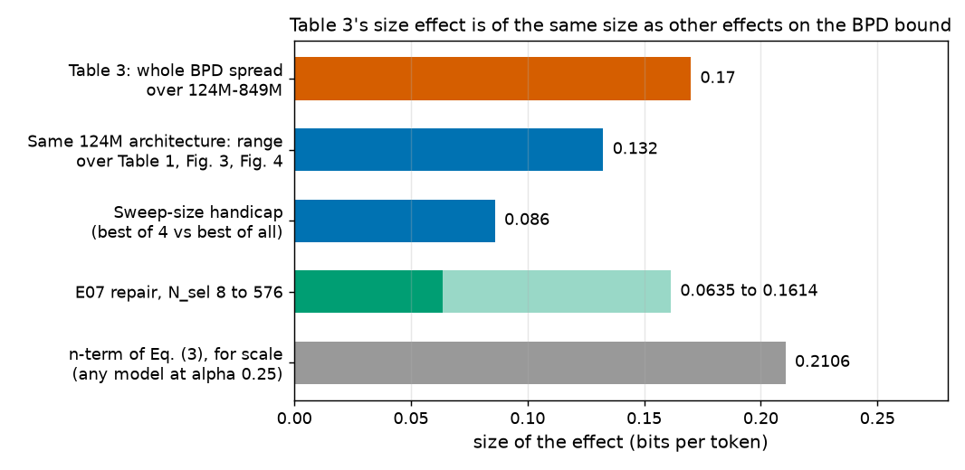
• Same architecture, three numbers. The 124M shape appears as 12.12 (Table 1), 12.007 (Figure 3) and 12.139 (Figure 4): a range of 0.132 with no explanation (errata E24, E39). Against Figure 3's 12.007, only 2 of 4 larger models win.
• Tuning handicap. The larger models had 4 training runs each (32 candidates with \(\alpha\)), the 124M model 72 (576 candidates) PAPER App. E, pp. 16–17. Chapter 26, using Figure 3's 10–12 trained models per size as a stand-in, estimates that the best of 4 runs is worse than the best of all of them by 0.086 bits/token on average. This works against the larger models, as the paper's own limitation note says PAPER §6.4, p. 7.
• E07 also favours the larger models once repaired. Repairing the n-term costs +0.1614 for the 124M grid (\(N_{\text{sel}} = 576\)) but +0.0986 for the larger-model grid (\(N_{\text{sel}} = 32\)), both at \(\Delta(0.25)\) (output [5]). A fair comparison would widen the BPD gap in their favour by 0.0628.
• No repeated runs. Without seeds or error bars (ranges showing how much a number moves when the experiment is rerun with a different seed), we cannot tell a 0.17 difference from run-to-run variation. The 0.132 same-architecture range is not that variation — it comes from different, unidentified runs or settings — but it shows that differences of this size arise without any change in model size.

Two corrections point in favour of the larger models; the same-architecture range and the lack of seeds point against any firm conclusion. The fair reading is "larger models are at least as good on BPD bounds", not "bounds improve with size". For top-1 and top-100, larger models are not better in Table 3; the top-1 improvement exists only along Figure 3's best line, below 125M parameters.

"More compressible" has a second problem: the winning models do not get smaller. In Figure 3 the best-BPD points sit at 3.89–9.94 KB with no trend in size (Chapter 26, output [5] there). What falls is the total code length of the data, which is training loss (C12).

One further point applies to all three columns: a lower upper bound does not by itself mean a lower true risk or a smaller generalization gap (deeper block "Ranking models by their bounds").

Summary of verdicts for abstract-level claims.

Abstract claim	Verdict	Main reason
First non-vacuous bounds for pretrained LLMs	Partly supported	True for compressed, smoothed SubLoRA models; original GPT-2's bound is 70.76
LLMs discover regularities that generalize	Partly supported	Certified model beats uniform guessing (12.12 < 15.62; ≥ 3.59 % top-1), but is weak (perplexity 1,478.6)
Bound valid for unbounded log-likelihood via smoothing	Supported (for the smoothed model)	Theorem A.2 correct; unsmoothed loss not bounded
Subsampling accelerates by orders of magnitude	Supported	768× (GPU-hours) or 96× (wall clock); 900× not derivable; cost 0.2106 bits/token
Non-vacuous bounds for nearly a billion parameters	Supported	849M: 12.01 < 15.62
Larger models: better bounds	Partly (BPD; top-1 below 125M) / not supported (top-100)	Non-monotone, spread 0.17 ≈ same-architecture range 0.132, no seeds; top-1 2 of 4 and top-100 0 of 4 in Table 3
Larger models: more compressible	Not supported as worded	Model size does not shrink; falling dataset code length is training loss

(c) What the paper genuinely achieves

Criticism is only useful next to an accurate account of what was done well.

• A real advance. PAPER §1–§2, pp. 1–4 The paper presents these as the first non-vacuous bounds for next-token prediction with transformer architectures of 124M–849M parameters. MY ANALYSIS We did not survey the literature to confirm priority. Within its scope, 12.12 bits/token against 15.62 is a genuine non-vacuous guarantee, and our recomputation reproduces it to 0.0022 (output [2]).
• A clean, honest framework. The finite-hypothesis bound with a compression prior (Eq. 1) needs no posterior distribution, no PAC-Bayes machinery and no assumption about the training algorithm. Every step is checkable, and the bits-versus-nats looseness it carries can only make bounds larger (E02).
• Two simple, correct devices. Prediction smoothing makes the unbounded log-loss usable at a modest price (the extra loss per token is at most \(\log_2\frac{1}{1-\alpha}\) = 0.415 bits at \(\alpha = 0.25\); Chapter 25, output [6] there). Subsampling costs only 0.2106 bits/token on the best bound. Both are correct, modulo the E07 selection issue, whose repair keeps every headline bound non-vacuous.
• An effective compressor for bounds. SubLoRA reaches 16.5 KB for a 124M-parameter architecture — 29,225 times smaller than float32 storage (output [1]) — while keeping enough fit for a non-vacuous bound, and it gives the best BPD bounds in every comparison reported.
• Reproducible headline number. The headline 12.12 (and the Figure 1–2 bounds) can be recomputed from the paper's own figures plus values recovered from the authors' public code. Other cells — the Original Model's 70.76, Table 3, Table 5 — cannot, because their sizes and empirical risks are not reported (errata E33, E53, E69). Our mini replication (Chapter 28) shows the whole method working end to end, with a bound of 4.347 above a true risk of 3.435 bits/char (output [9]).
• Candid limitations. PAPER §8, p. 9; §6.4, p. 7 The discussion names the most important restriction itself (bounds for already-trained models are future work), and §6.4 flags the unequal hyperparameter sweeps.

(d) Recommendations

What would make the broader claims convincing — each item is tied to a gap found above.

1. Seeds and error bars. Repeat each Table 3 configuration with at least three seeds and report the mean and the spread. Without this, differences of 0.17 bits/token cannot be interpreted.
2. Equal sweeps. Give every model size the same hyperparameter grid (same number of candidates), or report the best bound as a function of the number of runs.
3. Close E07. Either fix \(\alpha\) and \(d\) before drawing the subsample (for example, choose them on a second, independent subsample), or pay \(\ln N_{\text{sel}}\) in the n-term as shown in the first deeper block.
4. Decompose every bound. Report empirical risk, compressed size and both terms for every table cell (E33). This would settle C10 (Figure 4) and let readers check every number.
5. Report both kinds of average. Give per-document and per-token BPD for the same model, and say whether validation numbers use the smoothed or unsmoothed model (errata E28, E47).
6. Use the right baselines. For classification, compare with the majority-class error, not 50 % (E22).
7. Separate "better bound" from "better generalization". Report the gap \(R - \hat R\) estimated on held-out data for each model, next to the bound; a bound ranking alone cannot show that one model generalizes better.
8. Close the quality gap. Chapter 27 (output [4] there) computes that a model with GPT-2's validation loss would need to be described in at most 9,620,267 bits (1.15 MiB) for a non-vacuous document-level bound — 411 times smaller than float32. Showing that would certify a useful model.

Going deeper

Everything in this section is MY EXPLANATION unless tagged.

Going deeper: proof of the theorem chain, and exactly where each hypothesis is used

We prove the conclusion of "The theorem chain" from Hoeffding's inequality (proved in Chapter 9) and the union bound (proved in Chapter 10).

Step 1: one fixed hypothesis, the m-term. Fix \(h \in \mathcal H\). By (H3) the losses \(R(h, X_1), \dots, R(h, X_m)\) are independent, identically distributed, with mean \(R(h)\), and by (H2) each lies in an interval of width \(\Delta(h)\). Hoeffding's inequality gives, for every \(t > 0\),

\[ \Pr_X\big[R(h) - \hat R(h) > t\big] \le e^{-2mt^2/\Delta(h)^2}. \]

The probability is over the random draw of the \(m\) documents; \(h\) is fixed. Choose

\[ t_1(h) = \Delta(h)\sqrt{\frac{\ln\frac{1}{P(h)} + \ln\frac{1}{s\delta}}{2m}}, \]

so that \(e^{-2m t_1(h)^2/\Delta(h)^2} = P(h)\, s\delta\). (Check: \(2m t_1^2/\Delta^2 = \ln\frac1{P(h)} + \ln\frac1{s\delta}\), and \(e^{-(\ln a + \ln b)} = \frac{1}{ab}\) with \(a = 1/P(h)\), \(b = 1/(s\delta)\).)

Step 2: all hypotheses at once. Let \(A\) be the event "for every \(h \in \mathcal H\), \(R(h) \le \hat R(h) + t_1(h)\)". Its complement is the union over \(h\) of the failure events, so by the union bound

\[ \Pr[A^c] \le \sum_{h \in \mathcal H} P(h)\, s\delta \le s\delta, \]

using \(\sum_h P(h) \le 1\). This is where (H1) is essential: the prior must be fixed before the data, otherwise the sum is not over fixed events. Because \(A\) covers every \(h\), it also covers \(\hat h\), whichever \(h\) the training picks — including any choice of \(\alpha\), \(d\), \(r\) or learning rate made with the training data, as long as those choices are part of the description \(h\).

Step 3: the subsample, the n-term. Condition on the documents \(X = (X_1, \dots, X_m)\). Then \(\hat h\) is a fixed hypothesis (by (H5) it is a function of \(X\) only) and the numbers \(\ell_j = R(\hat h, X_j)\) are fixed. By (H4) the indices \(\sigma(i)\) are independent of \(X\) and uniform, so \(Y_i = \ell_{\sigma(i)}\) are i.i.d. with mean \(\frac1m\sum_j \ell_j = \hat R(\hat h)\), each in an interval of width \(\Delta(\hat h)\). Hoeffding again:

\[ \Pr_\sigma\big[\hat R(\hat h) - \hat{\hat R}(\hat h) > t \;\big|\; X\big] \le e^{-2nt^2/\Delta^2}. \]

Here the probability is over the random subsample only; the documents and \(\hat h\) are fixed. With \(t_2 = \Delta\sqrt{\ln\frac{1}{(1-s)\delta}/(2n)}\) the right side is \((1-s)\delta\). Call the success event \(B\). Since the conditional bound holds for every \(X\), averaging over \(X\) gives \(\Pr[B^c] \le (1-s)\delta\).

If the indices are drawn without replacement, the \(Y_i\) are dependent, but Hoeffding (1963, Theorem 4) shows that the exponential moments of their sum are no larger than with replacement; the same tail bound follows (proved in Chapter 17). This settles erratum E05.

Step 4: combine. On \(A \cap B\),

\[ R(\hat h) \le \hat R(\hat h) + t_1(\hat h) \le \hat{\hat R}(\hat h) + t_2 + t_1(\hat h), \]

which is Eq. (3). And \(\Pr[(A \cap B)^c] \le \Pr[A^c] + \Pr[B^c] \le s\delta + (1-s)\delta = \delta\). Both \(X\) and \(\sigma\) are random in this final statement.

Where (H5) fails, and the repair (E07). Suppose the reported model is chosen by comparing \(N\) candidates \(h_1(X), \dots, h_N(X)\) — each a function of the documents only — using their bounds computed on the subsample. Then \(\hat h = h_K\) where the index \(K\) depends on \(\sigma\), and Step 3 breaks: conditional on \(X\), \(\hat h\) is no longer fixed. Repair Step 3 by requiring the inequality for every candidate. Let \(B'\) be "for every \(k \le N\): \(\hat R(h_k) \le \hat{\hat R}(h_k) + t_2'(h_k)\)" with

\[ t_2'(h) = \Delta(h)\sqrt{\frac{\ln\frac{N}{(1-s)\delta}}{2n}}. \]

For each fixed \(k\) the conditional failure probability is at most \(e^{-\ln(N/((1-s)\delta))} = (1-s)\delta/N\); the union over \(N\) candidates gives \(\Pr[B'^c \mid X] \le (1-s)\delta\). Since \(\hat h\) is one of the candidates, \(B'\) implies the needed inequality for \(\hat h\) whatever \(K\) is, and Step 4 goes through unchanged. Each candidate may have its own width \(\Delta(h_k)\) (different \(\alpha\)), because the union step never uses the widths. The cost is the extra \(\ln N\) nats inside the n-term: +0.0635 to +0.1614 bits/token on the best model for \(N = 8\) to \(576\) (output [4]).

What the chain does not need. No assumption on the training algorithm, no assumption that tokens within a document are independent, and no assumption that the model is "good". What it does need, and cannot check, is (H3).

Going deeper: ranking models by their bounds

Several claims (C6, C7, C10) compare two models by their bounds. Here is what such a comparison can and cannot show.

Let \(b_A\) and \(b_B\) be valid bounds: \(\Pr[R(A) \le b_A] \ge 1-\delta\) and \(\Pr[R(B) \le b_B] \ge 1-\delta\), each over the random draw of the data that produced it. By the union bound both hold together with probability at least \(1 - 2\delta\). Suppose \(b_A < b_B\). On the event that both hold we know

\[ R(A) \le b_A, \qquad R(B) \le b_B . \]

Nothing here is a lower bound on \(R(B)\). So \(R(B)\) may be far below \(b_B\), and in particular below \(R(A)\). A smaller bound therefore does not imply a smaller true risk. To conclude \(R(A) < R(B)\) you need an upper bound on \(R(A)\) that is below a lower bound on \(R(B)\). A two-sided Hoeffding bound provides one: \(R(B) \ge \hat R(B) - t\) with the same kind of margin \(t\).

The same holds for the generalization gap \(R - \hat R\). The bound is \(\hat R + (\text{terms})\), and the terms are an upper bound on the gap, not an estimate of it.

A real example in which the ranking is reversed. In the mini replication (Chapter 28; our output [9], and Chapter 28's output for the training losses) the uncompressed "original" model has bound 9.48 bits/char (vacuous) and the SubLoRA model 4.347. Their true risks on 20,000 fresh documents are 1.488 and 3.435. The model with the much worse bound is much better, and both have training losses equal to their fresh-document losses to three decimals — neither model overfits. The difference in bounds comes entirely from the price of describing the model.

This is why "larger models have better bounds" does not by itself mean "larger models generalize better" or "regurgitate less" (C7): a bound difference can come from the empirical risk, from the compressed size, or from the luck of one run, and the paper reports neither the decomposition nor repeated runs.

Going deeper: the majority-class baseline for Table 5, derived

Erratum E22 says the right reference for a binary task with unequal classes is the error of the constant classifier that always answers the more common class.

SOURCE: Hugging Face datasets-server statistics for nyu-mll/glue, training splits QQP has 363,846 training pairs, 229,468 "not duplicate"; CoLA has 8,551 sentences, 6,023 "acceptable".

The constant classifier "always not duplicate" errs on the other 134,378 pairs: \(134{,}378/363{,}846 = 36.93\,\%\). For CoLA: \(2{,}528/8{,}551 = 29.56\,\%\).

How good a bound would that classifier get? It is one of two constant classifiers, so it can be named with 1 bit: \(\ln\frac1{P(h)} = \ln 2\) nats. Eq. (1) with \(\Delta = 1\), \(\delta = 0.05\) SOURCE: authors' code and \(m\) = 363,846 gives

\[ 0.3693 + \sqrt{\frac{\ln 2 + \ln 20}{2 \times 363{,}846}} = 0.3716 = 37.16\,\%, \]

and for CoLA (\(m\) = 8,551) 31.03 % (output [7]). The probability is over the random draw of the training examples; the classifier is fixed in advance. (We use the training-split class balance because the bound is about the training distribution; using the training error as \(\hat R\) is exact for a constant classifier.)

So the pretrained QQP bound, 35.27 %, beats even the bound of the constant classifier, 37.16 %. The pretrained CoLA bound, 38.89 %, is above the constant classifier's bound, 31.03 %: on CoLA, Table 5's best certificate is weaker than one any reader could compute for "always say acceptable".

Common misconceptions

• Misconception: The paper proves that GPT-2 generalizes. — Actually: it proves a bound for a compressed, smoothed model with perplexity about 1,479; the bound for the normally trained GPT-2 is 70.76 bits/token, which is vacuous. GPT-2's good generalization is shown by its held-out loss (4.35), not by any bound in the paper.
• Misconception: A vacuous bound means the model does not generalize. — Actually: it means this certificate is uninformative. The original GPT-2 has the best held-out loss in Table 2; in our mini replication the original model's bound is 9.48 while its true risk is 1.488, the best of all models.
• Misconception: If larger models have lower bounds, they must generalize better. — Actually: an upper bound says nothing about how far below it the truth lies; comparing true risks needs a lower bound on one of them, and comparing gaps needs a held-out estimate (deeper block "Ranking models by their bounds").
• Misconception: Erratum E07 invalidates the results. — Actually: it makes the published bounds slightly optimistic. The repaired best BPD bound is at most 12.2836 and the repaired top-1 bound at most 97.35 %, both still non-vacuous.
• Misconception: The i.i.d. assumption is guaranteed by sampling documents at random. — Actually: random sampling of the subsample is under the authors' control (H4). Whether the training documents are i.i.d. draws from a fixed process (H3) is an assumption about how OpenWebText came to exist, and the bound is only about that process (Chapter 15).
• Misconception: Table 3 shows a size trend because all four larger models beat 124M. — Actually: the 124M architecture itself appears with three different bounds spanning 0.132 bits/token; against Figure 3's 12.007 only 2 of 4 larger models win, and for top-100 error none does.

Self-test

Q1. The paper compared all 576 grid candidates on the same subsample for GPT-2 small. Using the E07 repair, what is the best model's BPD bound, and by how much does it exceed the published 12.12? Is it still non-vacuous?

Answer

The n-term becomes \(\Delta\sqrt{\ln\frac{576}{(1-s)\delta}/(2n)}\) with \(\Delta = 17.2020\), \(n = 10{,}000\), \(\delta = 0.05\) and \(m = 8{,}009{,}762\) SOURCE: authors' code / nanoGPT. Output [4] gives a bound of 12.2836 bits/token, 0.1614 above our reproduced 12.1222 (0.16 above the published 12.12). It is still below \(\log_2 V = 15.6170\), so still non-vacuous. The probability (at least 95 %) is over the random draw of the training documents and of the subsample; the 576 candidates are fixed functions of the training documents.

Q2. Model A has a BPD bound of 11.95 and model B one of 12.12, both valid at \(\delta = 0.05\). A colleague says: "So A generalizes better than B." What can you actually conclude, and what extra information would you need?

Answer

With probability at least \(1 - 2\delta = 0.90\) (union of the two failure events, over the random data behind each bound), \(R(A) \le 11.95\) and \(R(B) \le 12.12\). That does not order \(R(A)\) and \(R(B)\): \(R(B)\) could be far below 12.12. Nor does it order the generalization gaps, since each bound is an upper bound on the gap, not an estimate. To conclude \(R(A) < R(B)\) you need an upper bound on \(R(A)\) below a lower bound on \(R(B)\); to compare gaps you need held-out estimates of \(R - \hat R\) for both; and to separate the models from luck you need repeated runs. The Ch. 28 example (bounds 9.48 vs 4.347, true risks 1.488 vs 3.435) shows the ranking can be reversed.

Q3. Why does the abstract's claim "valid for the unbounded log-likelihood loss" need a qualification, and what is the qualification?

Answer

Hoeffding's inequality needs each loss to lie in a fixed interval of width \(\Delta\). The log-loss of an ordinary model is unbounded (a token of probability 0 costs infinitely many bits), so no finite \(\Delta\) exists. Prediction smoothing replaces the model by \(p_h = (1-\alpha)p_\theta + \alpha/V\), whose per-token loss lies between \(\log_2(V/\alpha) - \Delta\) and \(\log_2(V/\alpha)\) (Theorem A.2). The bound is therefore valid for the log-loss of the smoothed model, which is bounded by construction. It is not a bound on the unsmoothed model's log-loss.

Code for this chapter

Run it from the project root:

.venv/Scripts/python explainer/code/ch29_critique_numbers.py

Source: ch29_critique_numbers.py

"""Chapter 29 demo: every headline number used by the critique (Ch. 29) and by the home page (docs/index.md).

Claims reproduced / re-printed (recomputed with pacbound.py, or loaded from earlier outputs where the source data
are figure colours that only Ch. 26 decodes):
  [1] Home-page numbers: 124M parameters, float32 size (~4 billion bits), d <= 200,000, 16.5 KB, 95 % confidence,
      12.12 vs 15.62, 96.41 % vs 99.998 %, certified 3.6 %, 849M, 8 million documents, n = 10,000.
  [2] Table 1's 12.12 reproduced as 12.1222 from Fig. 2's best model (Eq. 3), and the KB / log-base checks (E35, E02).
  [3] What object is certified: Original Model 70.76 vs the largest possible smoothed loss; validation 10.53 vs 4.35
      bits/token and perplexities; certified accuracies (Table 1).
  [4] Validity gaps: E07 repair (union over N_sel candidates on the subsample) for BPD and top-1; subsampling cost.
  [5] Table 3 audit: spreads, monotonicity, Spearman rho with exact permutation p-values, wins over 124M (claim C6).
  [6] Figure 3 best-bound lines (exact, fig_extract.json); compressed-dataset bits per token (C12).
  [7] Figure 4 bars (C10); Table 5 vs majority-class baselines from the GLUE statistics (C9, E22).
  [8] Speed-up 900x vs 768x / 96x (C4, E19); SubLoRA vs Subspace top-1 frontier (C8).
  [9] Ch. 28 mini replication: bound vs true risk.
Assumptions not stated in the paper (labelled in the output): delta = 0.05, m = 8,009,762 documents [SOURCE: authors'
code / nanoGPT]; 1 KB = 8192 bits (E35); V = 50,257 [SOURCE: GPT-2 tokenizer].
Writes outputs/ch29_critique_numbers.txt and docs/assets/fig/ch29_effect_sizes.png.
"""
from __future__ import annotations

import itertools
import json
import math
import re
import sys
import time
from pathlib import Path

HERE = Path(__file__).resolve().parent
sys.path.insert(0, str(HERE))

import matplotlib  # noqa: E402

matplotlib.use("Agg")
import matplotlib.pyplot as plt  # noqa: E402

import pacbound as pb  # noqa: E402

ROOT = HERE.parent.parent
OUT = HERE / "outputs" / "ch29_critique_numbers.txt"
FIG = HERE.parent / "docs" / "assets" / "fig" / "ch29_effect_sizes.png"
T0 = time.time()
lines: list[str] = []


def say(s: str = "") -> None:
    print(s)
    lines.append(s)


M, N, DELTA, V = pb.M_DOCS, pb.N_SUB, pb.DELTA, pb.V_GPT2
KB = 8192  # bits per KB (E35)
FIGX = json.loads((HERE / "outputs" / "fig_extract.json").read_text(encoding="utf-8"))
CH28 = json.loads((HERE / "outputs" / "ch28_mini_sublora.json").read_text(encoding="utf-8"))
CH26 = (HERE / "outputs" / "ch26_table3_audit.txt").read_text(encoding="utf-8")


def fig2_left(key: str, d: int) -> float:
    return min(FIGX["figure2"]["left"][key], key=lambda p: abs(p["d"] - d))["value"]


def price_nats(c_bits: float, extra_bits: float = 0.0) -> float:
    return pb.log_inv_prior_nats_from_bits(c_bits, extra_bits)


say("Chapter 29 - headline numbers for the critique and the home page (ch29_critique_numbers.py)")
say(f"delta = {DELTA} [SOURCE authors' code]; m = {M:,} docs [SOURCE nanoGPT]; n = {N:,}; V = {V:,}; 1 KB = {KB} bits")

# ---------------------------------------------------------------- [1] home page
D124 = pb.gpt2_params(12, 768)
D849 = pb.gpt2_params(25, 1600)
f32 = 32 * D124
log2V = pb.random_guess_bpd()
top1_rand = pb.random_guess_topk_error(1)
say("[1] Home page (docs/index.md)")
say(f"  GPT-2 small D = {D124:,} params (~124 million); float32 = {f32:,} bits (~{f32/1e9:.2f} billion); "
    f"849M label = 25 x 1600 shape: {D849:,}")
say(f"  confidence 1 - delta = {100*(1-DELTA):.0f} %; documents m = {M:,} (~{M/1e6:.1f} million); subsample n = {N:,}; "
    f"largest d in the grid = {max(pb.D_GRID):,}")
c_bits = fig2_left("compressed_size_kb", 50000) * KB
say(f"  best model size {c_bits/KB:.4f} KB = {c_bits:,.0f} bits; float32 / best = {f32/c_bits:,.0f}x; "
    f"bits per GPT-2 parameter {c_bits/D124:.5f}")
say(f"  random guess: log2 V = {log2V:.4f} bits/token (paper 15.62); top-1 error 1 - 1/V = {100*top1_rand:.4f} % (paper 99.99)")

# ---------------------------------------------------------------- [2] reproduction
r_bpd = fig2_left("empirical_risk", 50000)
lo, hi, dlt = pb.smoothing_interval(0.25)
p0 = price_nats(c_bits)
t1, t2 = pb.eq3_terms(p0, M, N, width=dlt)
b0 = r_bpd + t1 + t2
b576 = pb.eq3_bound(r_bpd, price_nats(c_bits, math.log2(576)), M, N, width=dlt)
b8000 = pb.eq3_bound(r_bpd, price_nats(c_bits / KB * 8000), M, N, width=dlt)
b_bits_as_nats = pb.eq3_bound(r_bpd, c_bits + math.log2(576) + 2 * math.log2(c_bits + math.log2(576)), M, N, width=dlt)
assert abs(b0 - 12.12) < 0.005
say("[2] Table 1 BPD 12.12 from Fig. 2 (d = 50,000, alpha = 0.25), Eq. (3)")
say(f"  Rhathat {r_bpd:.4f} + m-term {t1:.4f} + n-term {t2:.4f} = {b0:.4f} bits/token (paper 12.12, diff {b0-12.12:+.4f}); "
    f"+log2 576 hyper bits: {b576:.6f}")
say(f"  Delta(0.25) = {dlt:.4f}; margin below log2 V = {log2V-b0:.4f}; share of bound: empirical {100*r_bpd/b0:.1f} %, "
    f"m-term {100*t1/b0:.1f} %, n-term {100*t2/b0:.1f} %")
say(f"  checks: 1 KB = 8000 bits -> {b8000:.4f}; bits plugged in as nats (E02/E52) -> {b_bits_as_nats:.4f} (conservative)")

# ---------------------------------------------------------------- [3] certified object
T1 = {"SubLoRA": (96.41, 77.90, 58.34, 12.12), "LoRA": (100, 84.37, 67.26, 13.09),
      "Subspace": (96.52, 79.36, 75.95, 14.59), "Original": (100, 100, 100, 70.76)}   # [PAPER Table 1]
T2_VAL = {"SubLoRA": 10.53, "LoRA": 11.21, "Subspace": 13.85, "Original": 4.35}          # [PAPER Table 2]
T4 = {"SubLoRA": (96.17, 78.18, 58.72, 12.09), "LoRA": (100, 85.85, 65.19, 12.90),
      "Subspace": (97.40, 80.15, 76.11, 14.68), "Original": (100, 100, 100, 65.37)}   # [PAPER Table 4]
max_loss = max(pb.smoothing_interval(a)[1] for a in pb.ALPHA_GRID)
say("[3] What is certified")
say(f"  Original Model bound 70.76 vs largest possible smoothed per-token loss log2(V/alpha) = {max_loss:.3f} (alpha 1e-4); "
    f"70.76 - log2 V = {70.76-log2V:.2f}")
ppl = {k: 2 ** v for k, v in T2_VAL.items()}
say(f"  validation BPD SubLoRA 10.53 vs Original 4.35 (diff {10.53-4.35:.2f}); perplexity 2^BPD: {ppl['SubLoRA']:,.1f} vs "
    f"{ppl['Original']:.1f} (ratio {ppl['SubLoRA']/ppl['Original']:.1f}x); at the bound 2^12.12 = {2**12.12:,.1f}; "
    f"uniform {V:,}")
cert = [100 - x for x in T1["SubLoRA"][:3]]
unif = [100 * k / V for k in (1, 10, 100)]
say(f"  certified accuracy SubLoRA top-1/10/100 = {cert[0]:.2f} / {cert[1]:.2f} / {cert[2]:.2f} % vs uniform "
    f"{unif[0]:.4f} / {unif[1]:.4f} / {unif[2]:.4f} % ({cert[0]/unif[0]:,.0f}x / {cert[1]/unif[1]:,.0f}x / {cert[2]/unif[2]:,.0f}x)")

# ---------------------------------------------------------------- [4] validity gaps
c1_bits = fig2_left("compressed_size_kb", 10000) * KB
r_top1 = min(FIGX["figure1"]["left_top1"]["points"]["SubLoRA"], key=lambda p: p["sum"])["train_risk"]
say("[4] Erratum E07: union over N_sel candidates compared on the same subsample (n-term uses ln(N_sel/((1-s) delta)))")
row_b, row_t = [], []
for ns in (1, 8, 32, 48, 576):
    bb = pb.eq3_bound(r_bpd, p0, M, N, width=dlt, n_selected=ns)
    bt = pb.eq3_bound(r_top1, price_nats(c1_bits), M, N, width=1.0, n_selected=ns)
    row_b.append(bb)
    row_t.append(bt)
    say(f"  N_sel = {ns:>3}: BPD bound {bb:.4f} ({bb-b0:+.4f}) | top-1 bound (d = 10,000 model, Rhathat {r_top1:.4f}) "
        f"{100*bt:.2f} % -> certified top-1 accuracy {100*(1-bt):.2f} %")
assert abs(100 * row_t[0] - 96.41) < 0.01
e07_lo, e07_hi = row_b[1] - b0, row_b[4] - b0
say(f"  Eq. (1) applied to the n = 10,000 subsample alone (no m-term): "
    f"{pb.eq1_bound(r_bpd, p0, N, width=dlt):.2f} bits/token (vacuous)")

# ---------------------------------------------------------------- [5] Table 3
SIZES = [124, 354, 458, 773, 849]
T3 = {"BPD": [12.12, 11.96, 11.95, 12.10, 12.01], "Top-1": [96.41, 95.99, 96.69, 96.17, 96.51],
      "Top-100": [58.34, 58.4, 58.49, 59.25, 58.89]}   # [PAPER Table 3]


def spearman(y):
    rk = sorted(range(len(y)), key=lambda i: y[i])
    r = [0] * len(y)
    for pos, i in enumerate(rk):
        r[i] = pos
    n = len(y)
    return 1 - 6 * sum((r[i] - i) ** 2 for i in range(n)) / (n * (n * n - 1))


say("[5] Table 3 [PAPER] (lower = better), sizes 124/354/458/773/849M")
spread_bpd = None
for k, y in T3.items():
    rho = spearman(y)
    perms = [spearman(list(p)) for p in itertools.permutations(y)]
    p_le = sum(r <= rho + 1e-12 for r in perms) / len(perms)
    steps = "".join("-" if b < a else "+" for a, b in zip(y, y[1:]))
    wins = sum(v < y[0] for v in y[1:])
    spread = max(y) - min(y)
    if k == "BPD":
        spread_bpd = spread
    say(f"  {k:7s}: steps {steps}; spread {spread:.2f}; larger beating 124M {wins}/4; diffs vs 124M "
        + ", ".join(f"{v-y[0]:+.2f}" for v in y[1:]) + f"; rho {rho:+.1f} (exact P(rho<=obs) {p_le:.3f})")
fig3_124 = FIGX["figure3"]["bpd_bound"]["best_line"][-1]["value"]
three_124 = (12.12, fig3_124, FIGX["figure4"]["bpd"]["regular"])
same_arch = max(three_124) - min(three_124)
say(f"  same 124M architecture: Table 1 12.12 vs Fig. 3 {fig3_124:.3f} (diff {fig3_124-12.12:+.3f}) vs Fig. 4 "
    f"{FIGX['figure4']['bpd']['regular']:.3f} (range {same_arch:.3f}); larger models beating Fig. 3's {fig3_124:.3f}: "
    f"{sum(v < fig3_124 for v in T3['BPD'][1:])}/4")
handicap = float(re.search(r"best of all: mean ([0-9.]+)", CH26).group(1))
nsel_large = pb.eq3_bound(r_bpd, p0, M, N, width=dlt, n_selected=32) - b0
say(f"  sweep-size handicap (ch26 output [3]): mean {handicap:.3f} bits/token; E07 repair at Delta(0.25): 124M grid "
    f"(N_sel 576) {e07_hi:+.4f} vs larger-model grid (N_sel 32) {nsel_large:+.4f} (difference {e07_hi-nsel_large:.4f})")

# ---------------------------------------------------------------- [6] Figure 3
say("[6] Figure 3 best-bound lines (exact from the PDF), 1.90M .. 124.75M parameters")
for key, lab, fmt_ in (("bpd_bound", "BPD  ", "{:.3f}"), ("top1_error_bound", "Top-1", "{:.4f}"),
                       ("compressed_dataset_size_bits", "data ", "{:.3e}")):
    ys = [p["value"] for p in FIGX["figure3"][key]["best_line"]]
    xs = [p["params"] for p in FIGX["figure3"][key]["best_line"]]
    steps = "".join("-" if b < a else "+" for a, b in zip(ys, ys[1:]))
    imin = min(range(len(ys)), key=lambda i: ys[i])
    say(f"  {lab}: " + " ".join(fmt_.format(v) for v in ys) + f" | steps {steps} | min at {xs[imin]/1e6:.2f}M")
data = [p["value"] for p in FIGX["figure3"]["compressed_dataset_size_bits"]["best_line"]]
kbmax = float(re.search(r"\.\.([0-9.]+) KB; max colour", CH26).group(1))
say(f"  data bits / {pb.OWT_TRAIN_TOKENS:,} tokens [SOURCE nanoGPT]: {data[0]/pb.OWT_TRAIN_TOKENS:.3f} -> "
    f"{data[-1]/pb.OWT_TRAIN_TOKENS:.3f} bits/token; model part <= {kbmax} KB (colourbar max, ch26) = "
    f"{kbmax*KB/data[-1]:.2e} of the total")

# ---------------------------------------------------------------- [7] Figure 4, Table 5
say("[7] Figure 4 bars (regular / permuted) and Table 5 vs class balance")
for k in ("bpd", "top1", "top100"):
    f4 = FIGX["figure4"][k]
    say(f"  Fig. 4 {k:6s}: {f4['regular']:.4f} / {f4['permuted']:.4f} (diff {f4['permuted']-f4['regular']:+.4f}; "
        f"+{100*(f4['permuted']/f4['regular']-1):.1f} %)")
T5 = {"qqp": (35.27, 71.72), "cola": (38.89, 53.42)}   # [PAPER Table 5]
for name in ("qqp", "cola"):
    st = json.loads((ROOT / "sources" / "ext" / f"glue_{name}_stats.json").read_text(encoding="utf-8"))
    freq = next(c for c in st["statistics"] if c["column_name"] == "label")["column_statistics"]["frequencies"]
    tot = sum(freq.values())
    maj_err = 100 * min(freq.values()) / tot
    const_bound = 100 * pb.eq1_bound(maj_err / 100, math.log(2), tot)
    pre, rnd = T5[name]
    say(f"  {name.upper():4s} train {tot:,} ({freq}): majority-class error {maj_err:.2f} %, its Eq. (1) bound (1 bit) "
        f"{const_bound:.2f} %; pretrained {pre} % ({pre-maj_err:+.2f} vs majority); random-init {rnd} %")

# ---------------------------------------------------------------- [8] speed-up, frontier, C8
say("[8] Speed-up (Section 1) and SubLoRA vs Subspace")
gpu_h = 3 * 24 * 8
say(f"  m/n = {M/N:.2f}; 3 days x 8 GPUs = {gpu_h} GPU-h vs 0.75 GPU-h -> {gpu_h/0.75:.0f}x "
    f"(log10 {math.log10(gpu_h/0.75):.2f}); wall clock 72 h / 0.75 h = {72/0.75:.0f}x (log10 {math.log10(96):.2f}); paper 900x")
pts = FIGX["figure1"]["left_top1"]["points"]
dom = sum(any(a["complexity"] <= b["complexity"] and a["train_risk"] <= b["train_risk"] for a in pts["SubLoRA"])
          for b in pts["Subspace"])
best = {k: min(p["sum"] for p in v) for k, v in pts.items()}
say(f"  Fig. 1 top-1: Subspace points dominated by a SubLoRA point {dom}/{len(pts['Subspace'])}; best bounds SubLoRA "
    f"{best['SubLoRA']:.4f} vs Subspace {best['Subspace']:.4f} (margin {best['Subspace']-best['SubLoRA']:.4f})")
cells = [(k, i) for k in ("LoRA", "Subspace") for i in range(4)]
say(f"  SubLoRA strictly best in Table 1 cells: {sum(T1['SubLoRA'][i] < T1[k][i] for k, i in cells)}/8; "
    f"Table 4: {sum(T4['SubLoRA'][i] < T4[k][i] for k, i in cells)}/8 (single runs)")

# ---------------------------------------------------------------- [9] Ch. 28
b28 = CH28["best"]
say("[9] Ch. 28 mini replication (synthetic text, bits/char; ch28_mini_sublora.json)")
say(f"  best SubLoRA bound {b28['bound']:.3f} (E07 {b28['bound07']:.3f}) vs true risk {b28['true']:.3f} "
    f"(+- {b28['true_hoeff']:.3f}); random guess {math.log2(CH28['V']):.3f}; original model bound "
    f"{CH28['original']['bound']:.2f} (vacuous) with true risk {CH28['original']['true']:.3f}")

# ---------------------------------------------------------------- figure
items = [
    ("Table 3: whole BPD spread\nover 124M-849M", spread_bpd, None, "#D55E00"),
    ("Same 124M architecture: range\nover Table 1, Fig. 3, Fig. 4", same_arch, None, "#0072B2"),
    ("Sweep-size handicap\n(best of 4 vs best of all)", handicap, None, "#0072B2"),
    ("E07 repair, N_sel 8 to 576", e07_lo, e07_hi, "#009E73"),
    ("n-term of Eq. (3), for scale\n(any model at alpha 0.25)", t2, None, "#999999"),
]
FMT = ["{:.2f}", "{:.3f}", "{:.3f}", "{:.4f}", "{:.4f}"]  # Table 3 is given to 2 decimals; Fig. 3/4 values to 3
fig, ax = plt.subplots(figsize=(8.2, 4.0))
for i, (lab, v, v2, col) in enumerate(items):
    ax.barh(i, v, color=col, height=0.6)
    if v2 is not None:
        ax.barh(i, v2 - v, left=v, color=col, alpha=0.4, height=0.6)
        ax.text(v2 + 0.004, i, f"{v:.4f} to {v2:.4f}", va="center", fontsize=10)
    else:
        ax.text(v + 0.004, i, FMT[i].format(v), va="center", fontsize=10)
ax.set_yticks(range(len(items)))
ax.set_yticklabels([it[0] for it in items], fontsize=10)
ax.invert_yaxis()
ax.set_xlabel("size of the effect (bits per token)", fontsize=11)
ax.set_xlim(0, 0.28)
ax.set_title("Table 3's size effect is of the same size as other effects on the BPD bound", fontsize=11)
ax.grid(axis="x", alpha=0.3)
fig.tight_layout()
FIG.parent.mkdir(parents=True, exist_ok=True)
fig.savefig(FIG, dpi=130)

say(f"figure: docs/assets/fig/{FIG.name}; all assertions passed")
OUT.parent.mkdir(parents=True, exist_ok=True)
OUT.write_text("\n".join(lines) + "\n", encoding="utf-8")
print(f"runtime {time.time()-T0:.1f} s (terminal only, so the output file is deterministic)")

Output:

Chapter 29 - headline numbers for the critique and the home page (ch29_critique_numbers.py)
delta = 0.05 [SOURCE authors' code]; m = 8,009,762 docs [SOURCE nanoGPT]; n = 10,000; V = 50,257; 1 KB = 8192 bits
[1] Home page (docs/index.md)
  GPT-2 small D = 123,689,472 params (~124 million); float32 = 3,958,063,104 bits (~3.96 billion); 849M label = 25 x 1600 shape: 849,009,600
  confidence 1 - delta = 95 %; documents m = 8,009,762 (~8.0 million); subsample n = 10,000; largest d in the grid = 200,000
  best model size 16.5325 KB = 135,434 bits; float32 / best = 29,225x; bits per GPT-2 parameter 0.00109
  random guess: log2 V = 15.6170 bits/token (paper 15.62); top-1 error 1 - 1/V = 99.9980 % (paper 99.99)
[2] Table 1 BPD 12.12 from Fig. 2 (d = 50,000, alpha = 0.25), Eq. (3)
  Rhathat 10.5945 + m-term 1.3171 + n-term 0.2106 = 12.1222 bits/token (paper 12.12, diff +0.0022); +log2 576 hyper bits: 12.122225
  Delta(0.25) = 17.2020; margin below log2 V = 3.4949; share of bound: empirical 87.4 %, m-term 10.9 %, n-term 1.7 %
  checks: 1 KB = 8000 bits -> 12.1067; bits plugged in as nats (E02/E52) -> 12.3871 (conservative)
[3] What is certified
  Original Model bound 70.76 vs largest possible smoothed per-token loss log2(V/alpha) = 28.905 (alpha 1e-4); 70.76 - log2 V = 55.14
  validation BPD SubLoRA 10.53 vs Original 4.35 (diff 6.18); perplexity 2^BPD: 1,478.6 vs 20.4 (ratio 72.5x); at the bound 2^12.12 = 4,451.3; uniform 50,257
  certified accuracy SubLoRA top-1/10/100 = 3.59 / 22.10 / 41.66 % vs uniform 0.0020 / 0.0199 / 0.1990 % (1,804x / 1,111x / 209x)
[4] Erratum E07: union over N_sel candidates compared on the same subsample (n-term uses ln(N_sel/((1-s) delta)))
  N_sel =   1: BPD bound 12.1222 (+0.0000) | top-1 bound (d = 10,000 model, Rhathat 0.9148) 96.41 % -> certified top-1 accuracy 3.59 %
  N_sel =   8: BPD bound 12.1857 (+0.0635) | top-1 bound (d = 10,000 model, Rhathat 0.9148) 96.78 % -> certified top-1 accuracy 3.22 %
  N_sel =  32: BPD bound 12.2208 (+0.0986) | top-1 bound (d = 10,000 model, Rhathat 0.9148) 96.98 % -> certified top-1 accuracy 3.02 %
  N_sel =  48: BPD bound 12.2304 (+0.1082) | top-1 bound (d = 10,000 model, Rhathat 0.9148) 97.04 % -> certified top-1 accuracy 2.96 %
  N_sel = 576: BPD bound 12.2836 (+0.1614) | top-1 bound (d = 10,000 model, Rhathat 0.9148) 97.35 % -> certified top-1 accuracy 2.65 %
  Eq. (1) applied to the n = 10,000 subsample alone (no m-term): 47.87 bits/token (vacuous)
[5] Table 3 [PAPER] (lower = better), sizes 124/354/458/773/849M
  BPD    : steps --+-; spread 0.17; larger beating 124M 4/4; diffs vs 124M -0.16, -0.17, -0.02, -0.11; rho -0.2 (exact P(rho<=obs) 0.392)
  Top-1  : steps -+-+; spread 0.70; larger beating 124M 2/4; diffs vs 124M -0.42, +0.28, -0.24, +0.10; rho +0.3 (exact P(rho<=obs) 0.742)
  Top-100: steps +++-; spread 0.91; larger beating 124M 0/4; diffs vs 124M +0.06, +0.15, +0.91, +0.55; rho +0.9 (exact P(rho<=obs) 0.992)
  same 124M architecture: Table 1 12.12 vs Fig. 3 12.007 (diff -0.113) vs Fig. 4 12.139 (range 0.132); larger models beating Fig. 3's 12.007: 2/4
  sweep-size handicap (ch26 output [3]): mean 0.086 bits/token; E07 repair at Delta(0.25): 124M grid (N_sel 576) +0.1614 vs larger-model grid (N_sel 32) +0.0986 (difference 0.0628)
[6] Figure 3 best-bound lines (exact from the PDF), 1.90M .. 124.75M parameters
  BPD  : 12.207 12.160 11.962 12.205 12.068 12.019 12.057 12.007 | steps --+--+- | min at 7.57M
  Top-1: 0.9761 0.9662 0.9630 0.9625 0.9641 0.9614 0.9600 0.9637 | steps ---+--+ | min at 82.34M
  data : 8.899e+10 8.955e+10 8.758e+10 8.751e+10 8.585e+10 8.568e+10 8.486e+10 8.503e+10 | steps +-----+ | min at 82.34M
  data bits / 9,035,582,198 tokens [SOURCE nanoGPT]: 9.849 -> 9.410 bits/token; model part <= 19.32 KB (colourbar max, ch26) = 1.86e-06 of the total
[7] Figure 4 bars (regular / permuted) and Table 5 vs class balance
  Fig. 4 bpd   : 12.1394 / 12.4520 (diff +0.3126; +2.6 %)
  Fig. 4 top1  : 0.9636 / 1.0122 (diff +0.0487; +5.1 %)
  Fig. 4 top100: 0.5922 / 0.6022 (diff +0.0100; +1.7 %)
  QQP  train 363,846 ({'not_duplicate': 229468, 'duplicate': 134378}): majority-class error 36.93 %, its Eq. (1) bound (1 bit) 37.16 %; pretrained 35.27 % (-1.66 vs majority); random-init 71.72 %
  COLA train 8,551 ({'unacceptable': 2528, 'acceptable': 6023}): majority-class error 29.56 %, its Eq. (1) bound (1 bit) 31.03 %; pretrained 38.89 % (+9.33 vs majority); random-init 53.42 %
[8] Speed-up (Section 1) and SubLoRA vs Subspace
  m/n = 800.98; 3 days x 8 GPUs = 576 GPU-h vs 0.75 GPU-h -> 768x (log10 2.89); wall clock 72 h / 0.75 h = 96x (log10 1.98); paper 900x
  Fig. 1 top-1: Subspace points dominated by a SubLoRA point 1/12; best bounds SubLoRA 0.9641 vs Subspace 0.9652 (margin 0.0011)
  SubLoRA strictly best in Table 1 cells: 8/8; Table 4: 8/8 (single runs)
[9] Ch. 28 mini replication (synthetic text, bits/char; ch28_mini_sublora.json)
  best SubLoRA bound 4.347 (E07 4.443) vs true risk 3.435 (+- 0.062); random guess 4.858; original model bound 9.48 (vacuous) with true risk 1.488
figure: docs/assets/fig/ch29_effect_sizes.png; all assertions passed