13. Kolmogorov complexity and the Solomonoff prior¶

Where this fits

Prerequisites: Chapter 12 (codes, prefix-free codes, the Kraft inequality, code → prior, Elias gamma, the length prior), Chapter 3 (bits, nats, \(\log_2\), \(\ln\)), the idea of a prior and Eq. (1) from Chapter 11, and "random initialization" and "seed" from Chapter 7. Used later by: Chapter 14 (compressed size as complexity), Chapter 23 and Chapter 29. Purpose: explain what the paper's "Solomonoff prior" and "Kolmogorov complexity \(K(h\mid\mathcal A)\)" mean, why \(K\) cannot be computed, and why the bound never needs it.

The problem this chapter solves¶

Everything in this section is MY EXPLANATION unless tagged.

Chapter 12 ended with a recipe. Fix a prefix-free code for models before you see any data. Give each model \(h\) the prior weight \(P(h) = 2^{-\ell(h)}\), where \(\ell(h)\) is the length of its codeword in bits. Then the complexity term of the bound is \(\ln\frac{1}{P(h)} = \ell(h)\ln 2\) nats.

A quick reminder of why this matters: the bound of Chapter 11 (Eq. 1) gets looser as \(\ln\frac{1}{P(h)}\) grows. So a code that gives the trained model a short codeword gives a tight bound.

But which code? There are endless codes. Each one favours different models. Is there a best one?

PAPER §4.1, p. 4 The paper answers by naming one: it adopts, following Lotfi et al. (2022), the "Solomonoff prior", built from the prefix Kolmogorov complexity \(K(h\mid A)\) of the model \(h\), with the architecture \(A\) given as input. It says \(K\) cannot be computed, and then bounds the complexity term by a compressed size \(C(h)\): \(\ln\frac1{P(h)} \le K(h\mid A)\ln 2 \le C(h)\ln 2 + 2\ln C(h)\) (the paper writes a bare "log"; Chapter 12 shows it must be \(\ln\) here, erratum E02).

MY EXPLANATION This chapter explains each piece of that sentence:

What a program and a description are, and what "the length of the shortest program that prints \(h\)" means.
Why the answer barely depends on the programming language (the invariance theorem).
Why nobody can compute it (incomputability), but every compressor gives an upper bound.
How it becomes a prior (the Solomonoff prior), and why its weights add up to at most 1.
The key point for the rest of the explainer: the bound never uses \(K\). Any fixed compression scheme already defines a valid prior by itself (Chapter 12). \(K\) is the motivating story: it explains why "short description" is the right thing to reward.

Intuition (and where the analogy breaks)¶

Everything in this section is MY EXPLANATION.

Describing a picture over the phone. You want a friend to draw exactly the picture you see. The picture is a 1000 × 1000 grid of black and white squares.

If it is a checkerboard, one sentence does it: "a checkerboard, 1000 squares a side, top-left black."
If it is TV static, there is no shortcut. You must read out all one million squares, one by one.

The shortest message that lets your friend rebuild the picture exactly is a measure of how complex the picture is. That is the idea of Kolmogorov complexity. Simple things have short descriptions. Patternless things do not.

Occam's razor. "Prefer the simplest explanation" becomes "prefer what has the shortest description". The Solomonoff prior turns this into numbers: every extra bit of description halves the prior weight.

Where it breaks.

The listener matters. "A checkerboard" is short only because your friend already knows the word. To someone who does not, you must first explain it. Kolmogorov complexity fixes the "listener" to be a computer running a fixed programming language. Switching languages changes the answer, but only by a fixed amount: the length of a dictionary (an interpreter) that translates one language into the other. That is the invariance theorem.
Nobody can find the shortest description. With pictures you can usually tell whether a description is short. In general you cannot: no program can compute the shortest description of every string (proved below).
"Looks random" is not "is random". TV static produced by a seeded pseudo-random generator (Chapter 7) has a short description: "static from generator G with seed 42". A compressor cannot see this; the true shortest description can. This is exactly the situation of a neural network's random initialization.

Precise definition¶

Everything in this section is MY EXPLANATION (standard definitions of algorithmic information theory; see Li & Vitányi, "An Introduction to Kolmogorov Complexity and Its Applications") unless tagged.

Programs and descriptions¶

Throughout, the objects we describe are binary strings (Chapter 12). A model \(h\) is turned into a binary string by some fixed rule (for example, list its numbers in a fixed order and write each in binary). So "the complexity of \(h\)" means the complexity of that string.

A computer (also called a machine) is a fixed procedure that reads an input string and follows instructions. It may eventually stop (halt) and leave an output string, or it may run forever.
A program for a computer \(U\) is an input string \(p\) that we feed to \(U\). We write \(U(p) = x\) if \(U\), run on \(p\), halts with output \(x\). The length \(|p|\) is measured in bits.
A description of \(x\) (relative to \(U\)) is any program \(p\) with \(U(p) = x\). A string has many descriptions: short clever ones and long dull ones.
A description language is the rule that says which strings are programs and what they print, that is, the choice of \(U\). Python 3 is an example.
A universal computer is one that can imitate every other computer. For each computer \(T\) there is a fixed string \(i_T\), an interpreter for \(T\), such that \(U(i_T\,p) = T(p)\) for every program \(p\): \(U\) reads the interpreter, then behaves like \(T\) on the rest of the input. Every general-purpose programming language is universal in this sense.

Kolmogorov complexity¶

The (plain) Kolmogorov complexity of a string \(x\) relative to \(U\) is the length of its shortest description:

\[ K^{\text{plain}}_U(x) = \min\{\, |p| \; : \; U(p) = x \,\} \quad \text{bits}. \]

In words: search all programs that print \(x\); the length of the shortest one is \(K^{\text{plain}}_U(x)\).

Prefix (self-delimiting) complexity¶

The plain definition has a defect for our purpose. A plain computer is told where its program ends (like a file with an end-of-file mark). That end marker carries information for free. As a result, the weights \(2^{-K^{\text{plain}}(x)}\) add up to infinity, so they cannot be a prior (proof in the Going-deeper block on \(Z\)).

The repair uses the prefix-free idea of Chapter 12.

A prefix machine reads its program one bit at a time from an input with no end marker. It must decide by itself when to stop reading. Its programs are therefore self-delimiting: each program marks its own end.
Consequence: the set of programs on which a prefix machine halts is a prefix-free set (proof in the first Going-deeper block).
The prefix Kolmogorov complexity of \(x\) is \(K_U(x) = \min\{\, |p| : U(p) = x \,\}\) where \(U\) is now a universal prefix machine. Units: bits.

From here on, "Kolmogorov complexity" and \(K\) mean the prefix version, as in the paper and the notation table.

Conditional complexity¶

The conditional Kolmogorov complexity \(K(x \mid y)\) is the length of the shortest program that prints \(x\) when the computer also receives \(y\) as a second input, for free. Information the listener already has costs nothing. Always \(K(x\mid y) \le K(x) + c\) for a constant \(c\) (a program may ignore \(y\)), and often \(K(x\mid y)\) is far smaller.

PAPER §4.1, p. 4 The paper conditions on the architecture: \(K(h \mid A)\), "with the model architecture \(A\) provided as input". (This explainer writes \(\mathcal A\) for the architecture, erratum E16.)

SOURCE: Lotfi et al. 2022, App. B The predecessor paper adds that its prior also conditions on the random seed that generates the initialization \(\theta_0\) and the projection matrix \(P\). SOURCE: Lotfi et al. 2022, §3 It also conditions on using the same compression and decompression method for every model in the prior.

MY EXPLANATION So in practice the "free" input \(y\) is everything fixed before training: the architecture, the seeds, the decompression program, the quantization scheme and the hyperparameter grid. (Quantization, which Chapter 21 makes precise, rounds each trained number to one of a few allowed values. The projection matrix \(P\) is the random matrix of Chapter 18.) Only what training changed has to be paid for in bits.

Four facts about K¶

Invariance theorem. For any two universal prefix machines \(U\) and \(V\) there is a constant \(c_{UV}\) such that \(|K_U(x) - K_V(x)| \le c_{UV}\) for every string \(x\). The constant is about the length of an interpreter of one machine written for the other. This is why one writes \(K(x)\) without naming \(U\): it is defined "up to an additive constant".
Most strings are incompressible (the counting argument). There are \(2^n\) strings of \(n\) bits, but fewer than \(2^{n-c}\) programs shorter than \(n - c\) bits. So fewer than a fraction \(2^{-c}\) of all \(n\)-bit strings have \(K(x) < n - c\). Such strings are called incompressible: no description is much shorter than the string itself.
Incomputability. No program can take any string \(x\) as input and output \(K(x)\). (Proof sketch via the Berry paradox in Going deeper.)
Every compressor gives an upper bound. Let \(E\) be any fixed, decodable compression scheme whose outputs form a prefix-free code, and let \(c_E\) be the length of a program for \(U\) that decodes it. Then \(K(x) \le \ell_E(x) + c_E\), where \(\ell_E(x)\) is the length of \(x\)'s compressed form. If the compressor's outputs are not prefix-free, add a length header (Chapter 12): \(K(x) \le C(x) + 2\lfloor \log_2 C(x)\rfloor + 1 + c_E\), where \(C(x)\) is the compressed length in bits.

Fact 4 is what makes \(K\) usable at all: it cannot be computed, but it can be bounded from above by running a compressor. The bound can be very loose (the worked example finds a factor of 12,370), and we can never tell how loose.

The Solomonoff (universal) prior¶

The universal prior (or Solomonoff prior) gives each hypothesis a weight that falls by half for every bit of its shortest description:

\[ P(h) = \frac{2^{-K(h \mid \mathcal A)}}{Z}, \qquad Z = \sum_{h'} 2^{-K(h' \mid \mathcal A)} . \]

Here \(K(h\mid\mathcal A)\) is in bits, and \(Z\), the normalizer, is the sum of the unnormalized weights over all hypotheses. Dividing by \(Z\) makes the weights add up to exactly 1.

\(Z \le 1\). The shortest programs of different hypotheses are different members of one prefix-free set, so by the Kraft inequality their weights \(2^{-K}\) add up to at most 1 (proof in Going deeper).
Therefore \(P(h) \ge 2^{-K(h\mid\mathcal A)}\): dividing by a number at most 1 can only make the weight larger.
Therefore, taking \(\ln\) of \(1/P(h) \le 2^{K(h\mid\mathcal A)}\):

\[ \ln\frac{1}{P(h)} \le K(h\mid\mathcal A)\,\ln 2 \ \text{nats}. \]

Occam's razor, quantified. A hypothesis with a 1,000-bit shortest description gets \(2^{-1000}/Z\); one with a 1,001-bit description gets half of that. A model "is simple" exactly when it has a short description given what the decoder already knows.

PAPER App. C, p. 15 The appendix writes the prior in this normalized form, \(P(h) = 2^{-K(h)}/Z\) (without the conditioning on \(A\)), and splits the cost of a model that includes hyperparameters, \(h = (\theta, d, r)\), as \(K(h) \le K(\theta \mid d, r) + K(d) + K(r)\). A hyperparameter chosen from \(N\) values listed in advance costs \(\log_2 N\) bits.

MY EXPLANATION That split holds up to an additive constant (erratum E12); the proof is in Going deeper.

Paper erratum E01: the prior inequality points the wrong way

PAPER §4.1, p. 4 The main text writes the Solomonoff prior as \(P(h) \le 2^{-K(h\mid A)}\) and in the next display concludes \(\ln\frac1{P(h)} \le K(h\mid A)\ln 2\).

MY EXPLANATION The conclusion does not follow from the stated inequality. From \(P(h) \le 2^{-K}\) one gets \(\frac1{P(h)} \ge 2^{K}\), so \(\ln\frac1{P(h)} \ge K\ln 2\): the opposite direction, and useless for an upper bound. The conclusion needs \(P(h) \ge 2^{-K(h\mid A)}\).

PAPER App. C, p. 15 SOURCE: Lotfi et al. 2022, §3 Both write \(P(h) = 2^{-K(h)}/Z\) with \(Z \le 1\), which gives exactly \(P(h) \ge 2^{-K(h)}\).

Corrected statement: \(P(h) = 2^{-K(h\mid\mathcal A)}/Z \ge 2^{-K(h\mid\mathcal A)}\), hence \(\ln\frac1{P(h)} \le K(h\mid\mathcal A)\ln 2\). No reported number changes.

Paper erratum E51: K is called 'prefix' but defined without the self-delimiting condition

PAPER §4.1, p. 4 The paper calls \(K\) the prefix Kolmogorov complexity, but the next sentence defines it as the length of the shortest program that produces \(h\) "for a fixed programming language \(P\)". That is the plain definition: it does not require programs to be self-delimiting. The same sentence also uses the letter \(P\) for the programming language, next to \(P(h)\) (the prior) and \(P\) (the projection matrix of §3 and §5).

MY EXPLANATION The difference matters for the prior. With plain complexity the weights \(2^{-K^{\text{plain}}(h)}\) add up to infinity (Going-deeper block on \(Z\)), so \(2^{-K}/Z\) cannot be formed. With the prefix version, \(Z \le 1\). SOURCE: Lotfi et al. 2022, §3 The predecessor paper's definition includes the condition (the shortest program that "also delimits itself").

Corrected reading: the shortest self-delimiting program for a fixed universal prefix machine. The paper's word "prefix" shows that this was intended; no number changes (erratum E51).

The paper's chain, and the shortcut the bound actually uses¶

PAPER §4.1, p. 4 The paper's full chain is

\[ \ln\frac{1}{P(h)} \;\le\; K(h\mid A)\ln 2 \;\le\; C(h)\ln 2 + 2\ln C(h), \]

where \(C(h)\) is the number of bits needed to represent \(h\) with a coding scheme specified in advance.

MY EXPLANATION The first inequality is the Solomonoff prior (with E01 corrected). The second is fact 4, except that fact 4 has a constant: the decoder length \(c_E\). Converted to nats, the paper's step drops \(c_E\ln 2\) (erratum E12, below). It also uses \(2\log_2 C\) for the header, where an Elias gamma header costs \(2\lfloor\log_2 C\rfloor + 1\) bits.

The shortcut. Skip \(K\) entirely. The compression scheme is fixed before the data, so by Chapter 12 it defines a prior directly. The length prior of Chapter 12, \(P(h) = C(h)^{-2}\,2^{-C(h)}\) for \(C(h) \ge 2\), adds up to at most 1 and gives

\[ \ln\frac{1}{P(h)} = C(h)\ln 2 + 2\ln C(h) \quad \text{exactly}. \]

No incomputable quantity appears and no constant is dropped. Everything the bound needs is computable.

So what is \(K\) for? It explains why compressed size is the right currency. By fact 4, the Solomonoff prior is at least as generous as every computable code prior, up to the constant factor \(2^{-c_E}\): no fixed compression scheme can beat it by more than a constant. In that sense "the shortest description" is the ideal. Any real compressor is an approximation of it that we can actually run.

Paper erratum E12: dropped constants in the step from K to C

PAPER §4.1, p. 4; App. C, p. 15 The step \(K(h\mid A)\ln 2 \le C(h)\ln 2 + 2\ln C(h)\) and the split \(K(h) \le K(\theta\mid d,r) + K(d) + K(r)\) are written without additive constants.

MY EXPLANATION Both hold only up to \(O(1)\): the first needs \(+\,c_E\ln 2\) nats for the length of the decoder (the second Going-deeper block below); the second needs the length of a small "glue" program (the last Going-deeper block). If the decoder is part of the conditioning information, as Lotfi et al. (2022) intend, \(c_E\) is only the length of an instruction "run the given decoder", which is small but not zero. The worked example shows what an unconditioned decoder would cost: a 1,024-byte decoder adds 5,678.26 nats, 5.0 % of a 20 KB model's complexity term.

The clean fix is the shortcut above: define the prior from the compression scheme itself. Then \(\ln\frac1{P(h)} = C\ln 2 + 2\ln C\) holds exactly (the length prior of Chapter 12; see the E12 entry on the errata page), and no Kolmogorov constant is needed.

Worked example with real numbers¶

Every number in this section is printed by ch13_zlib_kolmogorov.py (full output at the end of the chapter). Everything here is MY EXPLANATION.

Six strings and their descriptions¶

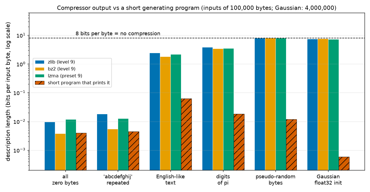
The script makes six inputs. Each one is printed by a short, complete Python program that uses only the standard library; the script runs each program in a fresh Python interpreter and keeps what it prints. It then compresses each input with three general-purpose compressors from Python's standard library: zlib (the method inside .zip and .png files), bz2 and lzma (the method inside .xz and .7z files), each at its strongest setting.

Input	Size (bytes)	zlib	bz2	lzma	Program that prints it	zlib bits per byte
all zero bytes	100,000	120	47	148	50	0.0096
"abcdefghij" repeated	100,000	228	69	160	56	0.0182
English-like text	100,000	30,275	22,806	27,392	777	2.4220
digits of \(\pi\)	100,000	48,174	43,229	43,732	230	3.8539
pseudo-random bytes	100,000	100,041	100,846	100,064	147	8.0033
Gaussian float32 "initialization"	4,000,000	3,716,054	3,797,647	3,684,644	295	7.4321

All sizes are in bytes (1 byte = 8 bits). The last column is \(8\times\) (zlib size)/(input size): 8 means "no compression at all".

What the inputs are:

English-like text: sentences of 4 to 12 words drawn from a list of 99 common English words, with common words more likely (word number \(r\) in the list has weight \(1/r\)). The randomness comes from a seeded pseudo-random generator.
Digits of \(\pi\): the first 100,000 decimal digits, 3141592653…, one byte per digit. The program uses the Gauss–Legendre iteration in whole-number arithmetic. The script checks the output twice: against a rerun with more guard digits (all 100,000 digits agree) and against Machin's classical formula (first 20,000 digits agree).
Pseudo-random bytes: 100,000 bytes from a 64-bit linear congruential generator with seed 1 (each new state is \(a\cdot x + b\) modulo \(2^{64}\); the output is the top byte).
Gaussian "initialization": 1,000,000 numbers drawn from the standard normal distribution by the same seeded generator, stored as 32-bit floating-point numbers (float32, 4 bytes each), like the starting weights of a neural network. Sample mean \(+0.0005\), standard deviation \(0.9994\).

What the table shows¶

Compressors find simple patterns. One hundred thousand zero bytes shrink to 47 bytes with bz2. The repeated pattern shrinks to 69 bytes. For these strings the compressors are about as good as a hand-written program (50 and 56 bytes). bz2 even beats the program slightly: Python and bz2 are different description languages, and the invariance theorem only promises agreement up to a constant.

Compressors find some structure in text. English-like text costs 2.4220 bits per character with zlib and 1.8245 with the best of the three. That is far below 8 bits, because frequent words and repeated phrases are cheap to refer back to.

Compressors miss deep structure completely. The digits of \(\pi\) cost 3.4583 bits per digit at best. A random digit carries \(\log_2 10 = 3.3219\) bits, so the compressors treat \(\pi\) as almost patternless. Yet a 230-byte program prints all 100,000 digits.

"Random-looking" is not "random". The pseudo-random bytes do not shrink at all: zlib's output (100,041 bytes) is slightly longer than the input, because of its own bookkeeping. The Gaussian initialization keeps 29.4772 of its 32 bits per number. Yet 147 and 295 bytes of program print them.

Upper bounds on K, side by side¶

A program text of \(b\) bytes is \(8b\) bits. To make it self-delimiting, put an Elias gamma length header in front (Chapter 12). This gives an upper bound on \(K\) relative to "Python 3 with its standard library" as the description language:

Input	Program bound on K (bits)	Best compressor (bits)	Compressor / program
digits of \(\pi\)	1,861	345,832	186×
pseudo-random bytes	1,197	800,328	669×
Gaussian initialization	2,383	29,477,152	12,370×

For example, the \(\pi\) program has 230 bytes \(= 1{,}840\) bits; \(\lfloor\log_2 1840\rfloor = 10\), so the gamma header is \(2\cdot 10 + 1 = 21\) bits, and the total is 1,861 bits.

Both columns are upper bounds on \(K\); the true \(K\) may be smaller still. But the comparison shows how far a good compressor can be from the shortest description: a factor of 12,370 for the Gaussian initialization.

Truly random strings: the counting argument in numbers¶

To zlib, pseudo-random data look like true randomness. The script compresses 1,000 pseudo-random strings of 1,000 bytes each (numpy generator, seed 0). Every output has 1,011 bytes; not one string got shorter.

For truly random strings no description language can do better. Take strings of \(n = 800{,}000\) bits (100,000 bytes). The fraction of them with \(K(x) < n - c\) is below \(2^{-c}\):

Saving \(c\)	Fraction of strings that can be compressed that much is below
8 bits (1 byte)	\(2^{-8} = 10^{-2.41}\)
80 bits (10 bytes)	\(2^{-80} = 10^{-24.08}\)
800 bits (100 bytes)	\(2^{-800} = 10^{-240.82}\)

At the other end, every 800,000-bit string can be printed literally, so \(K(x) \le 800{,}000 + 39\) bits \(+\) a constant (39 bits for the gamma header of 800,000). Almost all strings sit right at that ceiling.

Information given for free: conditional complexity¶

zlib can be handed a "preset dictionary" \(y\) that both compressor and decompressor know in advance. The compressed size of \(x\) with dictionary \(y\) imitates \(K(x\mid y)\):

String \(x\)	zlib alone (bytes)	zlib given \(y\) (bytes)
32,000 characters of the text, 10 characters changed; \(y\) = the original	10,297	293
8,000 float32 weights, 100 of them nudged; \(y\) = the unchanged "initialization"	29,702	864

The second row is the paper's situation in miniature. The initialization is given for free (it is regenerated from a seed). Only what training changed must be paid for.

Link to the paper¶

A model with 124 million parameters (PAPER Table 3, p. 8, the "124M" GPT-2-sized model) stored as raw float32 takes \(32 \times 124{,}000{,}000 = 3{,}968{,}000{,}000\) bits, which is 473.0 MiB. On our Gaussian sample the best compressor kept 92.12 % of the size, so a general compressor would not help much with a random initialization.
Given the generator, the initialization is described by its seed. SOURCE: authors' code, sublora_sublora_pipeline.py and sublora_nn_projectors.py The authors' code uses seed 137 for the model and for the projection. MY EXPLANATION In Elias gamma code, 137 takes 15 bits. And because the paper's prior conditions on the seed, even those bits are free.
MY EXPLANATION The 20 KB model of Chapter 12 has \(C = 163{,}840\) bits and \(C\ln 2 + 2\ln C = 113{,}589.25\) nats (computed with pacbound). If the decoder were not given for free, its length would enter the bound: a 1,024-byte decoder adds 5,678.26 nats (5.0 % of that), and a 1 MiB decoder adds 5,814,539.98 nats (5,118.9 %, more than fifty times the model's own cost). This is why the decoder belongs to the conditioning information, and why defining the prior directly from the code (the shortcut above) is the safe route.

SOURCE: authors' code, sublora_nn_create_model.py One practical note: the authors' bound-evaluation code reloads the saved random initialization from a checkpoint file instead of regenerating it from the seed. MY EXPLANATION That is a convenience, not a violation: what matters is that the initialization was fixed by a seed before seeing the data. Regenerating it exactly would need the same software (PyTorch's generator), which is precisely the "description language" that the invariance theorem says matters only up to a constant.

Going deeper¶

All proofs in this section are MY EXPLANATION (standard results of algorithmic information theory, written out) unless tagged. Notation: \(|p|\) is the length of a string in bits; "prefix-free", "Kraft inequality", "Elias gamma code" \(\gamma\) and the joining lemma are from Chapter 12. The blocks are ordered so that each one uses only earlier blocks.

Going deeper: why the halting programs of a prefix machine form a prefix-free set

Model. A prefix machine \(U\) has a one-way input tape holding an infinite sequence of bits. It reads bits one at a time, from left to right, and can never look back or ahead. We say \(U(p) = x\) if, when the tape begins with \(p\), the machine halts with output \(x\) after reading exactly the bits of \(p\) (no more, no fewer). The domain of \(U\) is the set of all such \(p\).

Claim. The domain is prefix-free.

Proof. Suppose \(p\) is in the domain and \(q = pu\) with \(u\) non-empty. Feed a tape that begins with \(q\). Its first \(|p|\) bits are exactly \(p\). The machine's behaviour up to the moment it has read \(|p|\) bits depends only on those bits, so it does exactly what it did on \(p\): it halts after reading exactly \(|p|\) bits. It never reads the bits of \(u\). So \(q\) is not read in full, and \(q\) is not in the domain. Hence no member of the domain is a proper prefix of another member. ∎

Consequence (Kraft). By the Kraft inequality, \(\sum_{p \in \text{domain}} 2^{-|p|} \le 1\). (The domain is usually infinite; Chapter 12's limit argument covers that case.)

Python files are not like this. A Python program is read up to the end of the file, so the file's end marks the program's end for free. Python is a "plain" description language. To turn a Python program into a self-delimiting one, put an Elias gamma header with its length in front; for the 1,840-bit \(\pi\) program this costs 21 bits.

Going deeper: three upper bounds on K (literal printing, any compressor, and the header)

(a) Literal printing. Let \(T_{\text{lit}}\) be the prefix machine that reads \(\gamma(n)\), learns \(n\), then reads exactly \(n\) more bits and prints them. Its domain \(\{\gamma(n)\,x : |x| = n\}\) is prefix-free (joining lemma). With an interpreter \(i_{\text{lit}}\) for \(U\):

\[ K(x) \le |i_{\text{lit}}| + |\gamma(|x|)| + |x| = |x| + 2\lfloor\log_2|x|\rfloor + 1 + c_{\text{lit}} . \]

For a 100,000-byte string this is \(800{,}000 + 39\) bits plus the constant.

(b) Any prefix-free compressor. Let \(E\) be a compression scheme fixed in advance whose outputs \(E(x)\) form a prefix-free code, with a decoder that reads \(E(x)\) bit by bit and prints \(x\). That decoder is a prefix machine \(T_E\) with \(T_E(E(x)) = x\). With its interpreter \(i_E\):

\[ U(i_E\, E(x)) = T_E(E(x)) = x \quad\Longrightarrow\quad K(x) \le |E(x)| + |i_E| = \ell_E(x) + c_E . \]

(c) A compressor whose outputs are not prefix-free (zlib, or the arithmetic coder of Chapter 22, which turns a list of symbols into a near-minimal number of bits). Put \(\gamma(C(x))\) in front, where \(C(x)\) is the compressed length in bits. Chapter 12 proved that the result is prefix-free. Applying (b):

\[ K(x) \le C(x) + 2\lfloor\log_2 C(x)\rfloor + 1 + c_E \ \text{bits}. \]

Multiply by \(\ln 2\) to get nats: \(K(x)\ln 2 \le C\ln 2 + 2\lfloor\log_2 C\rfloor\ln 2 + (1 + c_E)\ln 2 \le C\ln 2 + 2\ln C + (1 + c_E)\ln 2\), using \(\lfloor\log_2 C\rfloor \le \log_2 C\) and \(\log_2 C \cdot\ln 2 = \ln C\). Compared with the paper's \(C\ln 2 + 2\ln C\), the extra term is \((1 + c_E)\ln 2\): this is erratum E12.

Conditional version. Everything above holds with \(\mathcal A\) given to all machines. If the decoder itself is part of the given information, \(i_E\) shrinks to a fixed instruction "run the decoder you were given on the rest of the tape", whose length does not depend on the decoder.

Going deeper: the invariance theorem (proof sketch)

Theorem. Let \(U\) and \(V\) be universal prefix machines. There is a constant \(c_{UV}\) such that for every string \(x\), \(|K_U(x) - K_V(x)| \le c_{UV}\).

Proof. Because \(U\) is universal, it has an interpreter \(i_V\) for \(V\): \(U(i_V\,p) = V(p)\) for every \(p\) in the domain of \(V\). Let \(p^\ast\) be a shortest \(V\)-program for \(x\), so \(|p^\ast| = K_V(x)\). Then \(i_V\,p^\ast\) is a \(U\)-program for \(x\), so

\[ K_U(x) \le |i_V| + |p^\ast| = K_V(x) + |i_V| . \]

Since \(V\) is universal too, the same argument with the roles swapped gives \(K_V(x) \le K_U(x) + |i_U|\). Together, \(|K_U(x) - K_V(x)| \le \max(|i_U|, |i_V|) =: c_{UV}\). The constant depends on the two machines, but not on \(x\). ∎

What is skipped. That a universal prefix machine exists. The standard construction lists all prefix machines \(T_1, T_2, \ldots\) (every machine can be converted into one that behaves as a prefix machine), lets \(U\) read \(\gamma(i)\) and then imitate \(T_i\); the domain \(\{\gamma(i)\,p\}\) is prefix-free by the joining lemma. The conversion step needs a formal model of computation (Turing machines) and is in Li & Vitányi, §3.1.

How large is the constant? It can be large: the length of a complete Python interpreter, or of PyTorch's random generator. For long strings it is negligible; for short strings it can dominate. This is one reason why the explainer prefers a prior defined by a concrete code fixed in advance, where no such constant appears.

Going deeper: the counting argument (most strings are incompressible)

Claim. For whole numbers \(n \ge 1\) and \(0 \le c \le n\), fewer than \(2^{n-c}\) strings \(x\) (of any length) have \(K(x) < n - c\). Hence among the \(2^n\) strings of length \(n\), the fraction with \(K(x) < n - c\) is below \(2^{-c}\).

Proof. The number of binary strings of length \(j\) is \(2^j\). The number of strings of length less than \(L = n - c\) is

\[ \sum_{j=0}^{L-1} 2^j = 2^L - 1 < 2^{n-c}, \]

by the geometric sum (\(2^0 + 2^1 + \cdots + 2^{L-1} = 2^L - 1\), which one checks by adding 1 and doubling repeatedly). Each program prints at most one string, so at most \(2^{n-c} - 1\) strings have a program shorter than \(n - c\), that is, have \(K(x) < n - c\). Divide by the \(2^n\) strings of length \(n\): \((2^{n-c} - 1)/2^n < 2^{-c}\). ∎

The argument never used anything about \(U\) except that each program has one output, so it holds for plain and prefix complexity and for every description language. (For prefix machines, Kraft makes the count even smaller.)

In probability language. Draw an \(n\)-bit string uniformly at random; what is random is the string, what is fixed is \(U\), \(n\) and \(c\). Then \(\Pr[K(x) < n - c] < 2^{-c}\). SOURCE: Lotfi et al. 2022, App. A.1 The predecessor paper uses this argument to show that a model which fits randomly labelled data cannot be compressed much.

At least one string of each length is fully incompressible. With \(c = 0\): fewer than \(2^n\) strings have \(K < n\), but there are \(2^n\) strings of length \(n\). So some \(n\)-bit string has \(K(x) \ge n\).

Going deeper: K cannot be computed (the Berry paradox, made rigorous)

The paradox. "The smallest number that cannot be described in fewer than twenty words" has just been described in fewer than twenty words. In ordinary language this is a puzzle. With programs it becomes a proof.

Theorem. There is no program that, given any string \(x\), halts and outputs \(K(x)\).

Proof sketch. Suppose such a program existed. Use it to build, for each whole number \(n\), the following prefix program \(Q_n\):

read \(\gamma(n)\) from the tape, to learn \(n\);
go through all strings in order (by length, then alphabetically: empty string, 0, 1, 00, 01, …);
for each string \(x\), compute \(K(x)\) with the assumed program;
print the first \(x\) with \(K(x) \ge n\), and halt.

\(Q_n\) halts. By the counting argument, fewer than \(2^n\) strings have \(K < n\), while there are infinitely many strings; so step 4 is reached. Call its output \(x_n\). By construction,

\[ K(x_n) \ge n . \]

But \(Q_n\) itself is a description of \(x_n\). Its length is \(c_0\) bits for the fixed instructions of steps 2–4 (which do not depend on \(n\)) plus \(2\lfloor\log_2 n\rfloor + 1\) bits for \(\gamma(n)\). So

\[ K(x_n) \le c_0 + 2\lfloor\log_2 n\rfloor + 1 . \]

The right side grows like \(2\log_2 n\), the left side at least like \(n\). For large \(n\), \(c_0 + 2\lfloor\log_2 n\rfloor + 1 < n\), and the two displays contradict each other. So the assumed program cannot exist. ∎

How large is "large"? The script computes the smallest such \(n\). If the search instructions take \(c_0 = 8{,}000\) bits (1,000 bytes), the contradiction appears at \(n = 8{,}026\): a 1,000-byte program would be printing a string whose shortest description is at least 8,026 bits. For \(c_0 = 80{,}000\) bits it appears at \(n = 80{,}034\).

What is skipped. A formal model of computation, and the check that steps 2–4 can be written as a prefix program of fixed length. Both are routine once Turing machines are defined.

Where the difficulty lives: the halting problem. The halting problem asks for a program that decides, for any program and input, whether it eventually halts; Turing proved that none exists. Computing \(K(x)\) would require knowing that every shorter program either never halts or prints something else, which runs into the same wall.

What can be done. Run all programs in parallel, giving each a few more steps in every round. Whenever a program halts with output \(x\), record its length. The recorded minimum only decreases, and it eventually reaches \(K(x)\). But we can never know that it has stopped decreasing. This is why \(K\) is said to be approximable from above: every compressor, and every program we write, is one such upper bound.

Going deeper: Z ≤ 1, P(h) ≥ 2^(−K), and why the plain version fails

Setting. \(U\) is a universal prefix machine that also receives \(\mathcal A\); hypotheses are strings (models encoded by a fixed rule). For each \(h\) let \(p_h\) be a shortest program with \(U(p_h \mid \mathcal A) = h\) (if several have the same length, take the alphabetically first). So \(|p_h| = K(h\mid\mathcal A)\).

Claim 1: \(0 < Z \le 1\). Different hypotheses have different shortest programs: a program has only one output, so \(p_h = p_{h'}\) would force \(h = h'\). All the \(p_h\) lie in the domain of \(U(\cdot\mid\mathcal A)\), which is prefix-free (first block). A subset of a prefix-free set is prefix-free, so by the Kraft inequality

\[ Z = \sum_h 2^{-K(h\mid\mathcal A)} = \sum_h 2^{-|p_h|} \le 1 . \]

\(Z > 0\) because every string has some program (block on upper bounds, part (a)), so each term is positive. ∎

Claim 2: the complexity term. From \(0 < Z \le 1\) we get \(\ln Z \le 0\), and

\[ \begin{aligned} \ln\frac{1}{P(h)} &= \ln\frac{Z}{2^{-K(h\mid\mathcal A)}} \\ &= K(h\mid\mathcal A)\ln 2 + \ln Z \\ &\le K(h\mid\mathcal A)\ln 2 \ \text{nats}. \end{aligned} \]

The first line uses \(1/P(h) = Z\,2^{K}\); the second uses \(\ln(ab) = \ln a + \ln b\) and \(\ln 2^{K} = K\ln 2\). Equivalently \(P(h) \ge 2^{-K(h\mid\mathcal A)}\), which is erratum E01's corrected direction.

Claim 3: the plain version cannot be normalized. Let \(T\) be a plain machine that prints its whole program (it knows where the program ends). With an interpreter of length \(c\), every \(n\)-bit string has \(K^{\text{plain}}(x) \le n + c\), so \(2^{-K^{\text{plain}}(x)} \ge 2^{-n-c}\). Sum over the \(2^n\) strings of length \(n\), then over all \(n\):

\[ \sum_x 2^{-K^{\text{plain}}(x)} \ge \sum_{n \ge 0} 2^n \cdot 2^{-n-c} = \sum_{n\ge0} 2^{-c} = \infty . \]

So "\(2^{-K^{\text{plain}}}/Z\)" has \(Z = \infty\) and is not a prior. Only the prefix version works.

Solomonoff's own construction. Solomonoff (1964) weighted every program for \(h\), not only the shortest. In its discrete form this is the universal distribution \(m(h) = \sum_{p \,:\, U(p) = h} 2^{-|p|}\). Kraft on the whole domain gives \(\sum_h m(h) \le 1\), and keeping only the shortest program gives \(m(h) \ge 2^{-K(h)}\), so the same bound \(\ln\frac1{m(h)} \le K(h)\ln 2\) holds. The coding theorem (Levin 1974; Chaitin 1975) shows that, conversely, \(-\log_2 m(h) \ge K(h) - c\) for a constant \(c\), so the two versions differ by at most a constant number of bits. We do not need it; its proof is in Li & Vitányi, §4.3.

Going deeper: the Solomonoff prior beats every fixed code, up to a constant

Claim. Let \(E\) be any prefix-free code on hypotheses that a program can decode, fixed in advance, with code prior \(P_E(h) = 2^{-\ell_E(h)}\). Then for every \(h\),

\[ P(h) \ge 2^{-K(h\mid\mathcal A)} \ge 2^{-\ell_E(h) - c_E} = 2^{-c_E}\,P_E(h) . \]

Proof. The first step is Claim 2 of the previous block; the second is the compressor bound \(K \le \ell_E + c_E\). ∎

In words: up to the fixed factor \(2^{-c_E}\), the universal prior gives every hypothesis at least as much weight as any computable code does. This is the precise sense in which "shortest description" is the ideal.

Why the bound should still use \(P_E\). To compute a bound with the universal prior we need a number that is at least \(\ln\frac1{P(h)}\). The best computable one available is \(K\ln 2 \le (\ell_E(h) + c_E)\ln 2\). With \(P_E\) itself the term is exactly \(\ell_E(h)\ln 2\). So, for any bound we can actually evaluate, using the code prior directly is better by \(c_E\ln 2\) nats and is never worse. The universal prior would only help if \(K(h)\) were much smaller than \(\ell_E(h)\), and incomputability means we could never certify that.

Going deeper: the App. C split K(θ, d, r) ≤ K(θ | d, r) + K(d) + K(r) + O(1)

Claim. For strings \(\theta, d, r\) (with the pair or triple encoded by a fixed rule),

\[ K(\theta, d, r) \le K(\theta \mid d, r) + K(d) + K(r) + c . \]

Proof. Let \(p_d\) and \(p_r\) be shortest programs for \(d\) and \(r\), and \(p_\theta\) a shortest program that prints \(\theta\) when given \((d, r)\). Build the program \(g\,p_d\,p_r\,p_\theta\), where \(g\) is a fixed "glue" program of \(c\) bits that does the following: run the self-delimiting program that follows and save its output \(d\); do the same for \(r\); run the next self-delimiting program with \((d, r)\) as its free input, to get \(\theta\); print the encoded triple. The glue knows where each part ends because each part is self-delimiting (prefix-free), with no separators needed (joining lemma of Chapter 12). The length is \(c + K(d) + K(r) + K(\theta\mid d, r)\). ∎

This is exactly where the self-delimiting property earns its keep: with plain programs the glue could not tell where \(p_d\) ends and \(p_r\) begins.

The \(\log_2 N\) bits for a hyperparameter. PAPER App. C, p. 15 If \(d\) is one of \(N\) values listed in advance, its encoding costs \(\log_2 N\) bits. MY EXPLANATION With the list given to the decoder, the index of \(d\) in a fixed-length code costs \(\lceil\log_2 N\rceil\) bits (Chapter 12), so \(K(d \mid \text{list}) \le \lceil\log_2 N\rceil + c\). Indexing the whole grid of combinations at once avoids rounding up separately for each hyperparameter; Chapter 24 counts these bits for the paper's grid. As erratum E12 notes, the paper writes these inequalities without the constant \(c\).

Common misconceptions¶

Everything in this section is MY EXPLANATION.

Misconception: "The paper computes the Kolmogorov complexity of its models." — Actually: \(K\) cannot be computed by any program. The paper computes a compressed size \(C(h)\), and the bound can be justified from \(C(h)\) alone, with a prior defined by the compression scheme (Chapter 12).
Misconception: "The zlib size of a file is its Kolmogorov complexity." — Actually: it is only an upper bound (plus a decoder constant), and it can be very loose: 100,000 digits of \(\pi\) need 345,832 bits with the best of three compressors but at most 1,861 bits as a Python program.
Misconception: "Data that a compressor cannot shrink are random and have high complexity." — Actually: pseudo-random bytes and a seeded Gaussian initialization do not shrink at all, yet 147 and 295 bytes of program print them. Incompressible-by-zlib is not incompressible.
Misconception: "Because \(K\) depends on the programming language, it is arbitrary." — Actually: two universal languages give complexities that differ by at most a constant that does not depend on the string (the invariance theorem). The constant can matter for short strings, which is one more reason to use a concrete code fixed in advance.
Misconception: "The bound is valid only if one uses the true Solomonoff prior." — Actually: any prior fixed before the data works. A fixed compression scheme gives a valid prior directly and, for any bound that can actually be computed, a tighter one.
Misconception: "A 124M-parameter model must have a huge description, because its random initialization alone is 3,968,000,000 bits." — Actually: the initialization is regenerated from a seed that the prior conditions on, so it costs nothing. Only the trained, compressed part is paid for.

Self-test¶

Q1. (numeric) Strings of 100,000 bytes are drawn uniformly at random. Give an upper bound on the probability that a string can be described by a program at least 10 bytes shorter than itself. What is random and what is fixed in this statement?

Answer

\(n = 800{,}000\) bits and \(c = 80\) bits. The counting argument gives \(\Pr[K(x) < n - 80] < 2^{-80} = 10^{-24.08}\) (script block [4]). Random: the string \(x\). Fixed: the universal machine \(U\), the length \(n\) and the saving \(c\). (The bound holds for every description language, because the proof only counts programs.)

Q2. (conceptual) Section 4.1 writes \(P(h) \le 2^{-K(h\mid A)}\) and then concludes \(\ln\frac1{P(h)} \le K(h\mid A)\ln 2\). What is wrong, and what is the correct statement and its justification?

Answer

From \(P(h) \le 2^{-K}\) one only gets \(\ln\frac1{P(h)} \ge K\ln 2\), the wrong direction (erratum E01). The correct prior is \(P(h) = 2^{-K(h\mid\mathcal A)}/Z\) with \(Z = \sum_{h'} 2^{-K(h'\mid\mathcal A)}\). Shortest self-delimiting programs of different hypotheses form a prefix-free set, so \(Z \le 1\) by the Kraft inequality. Hence \(P(h) \ge 2^{-K(h\mid\mathcal A)}\) and \(\ln\frac1{P(h)} = K\ln 2 + \ln Z \le K\ln 2\). With plain (not self-delimiting) complexity \(Z\) would be infinite, which is why "prefix" matters.

Q3. (numeric and conceptual) A colleague proposes to bound \(\ln\frac1{P(h)}\) by going through \(K\): "our decoder is a 1,024-byte program not given to the prior, so \(\ln\frac1{P(h)} \le (C + 2\log_2 C + 8 \cdot 1024)\ln 2\)." For the 20 KB model (\(C = 163{,}840\) bits), how many nats does the decoder add? What is the better option?

Answer

\(8 \times 1024 = 8{,}192\) bits, times \(\ln 2\): 5,678.26 nats, which is 5.0 % of the model's own \(C\ln 2 + 2\ln C = 113{,}589.25\) nats (script block [7]). Better: fix the compression scheme (including the decoder) before seeing data and use its own prior, the length prior \(P(h) = C^{-2}2^{-C}\) of Chapter 12. Then \(\ln\frac1{P(h)} = C\ln 2 + 2\ln C\) exactly, and the decoder costs nothing, because it is part of the prior, not of the message.

Code for this chapter¶

Run it from the project root:

.venv/Scripts/python explainer/code/ch13_zlib_kolmogorov.py

Source: ch13_zlib_kolmogorov.py

"""Chapter 13 demo: Kolmogorov-complexity intuition with real compressors (zlib, bz2, lzma).

What this script reproduces or illustrates (every number quoted in Chapter 13 comes from here):
  1. A compressor's output length is an upper bound on Kolmogorov complexity (up to the length of the
     decompressor). Six inputs, each PRINTED BY A SHORT PYTHON PROGRAM (run in a fresh interpreter),
     are compressed with zlib (level 9), bz2 (level 9) and lzma (preset 9). Structured inputs shrink a
     lot; pi digits, pseudo-random bytes and a seeded Gaussian "random initialization" do not, although
     the programs that print them are a few hundred bytes long (compressor size >> K).
  2. Bits per symbol: pi digits vs log2 10; English-like text per character; float32 Gaussian vs 32.
  3. Pseudo-random strings do not shrink under zlib (1,000 strings of 1,000 bytes, numpy seed 0).
  4. The counting argument: fewer than 2^(n-c) programs are shorter than n - c bits, so fewer than a
     2^-c fraction of n-bit strings can be compressed by c or more bits.
  5. Conditional complexity K(x|y), imitated with zlib's preset dictionary: an edited text given the
     original, and perturbed weights given their initialization.
  6. The arithmetic behind the Berry-paradox proof that K is incomputable.
  7. Link to the paper (sec. 4.1, App. C): raw size of a 124M-parameter float32 model; the seed;
     the cost of a decompressor constant (erratum E12) vs the direct code prior of pacbound.
Figure: docs/assets/fig/ch13_compression_bars.png
Output: code/outputs/ch13_zlib_kolmogorov.txt
"""
from __future__ import annotations

import bz2
import lzma
import math
import subprocess
import sys
import time
import zlib
from math import isqrt
from pathlib import Path

import numpy as np
import matplotlib

matplotlib.use("Agg")
import matplotlib.pyplot as plt  # noqa: E402

HERE = Path(__file__).resolve().parent
sys.path.insert(0, str(HERE))
import pacbound as pb  # noqa: E402

OUT_TXT = HERE / "outputs" / "ch13_zlib_kolmogorov.txt"
FIG_DIR = HERE.parent / "docs" / "assets" / "fig"
OUT_TXT.parent.mkdir(parents=True, exist_ok=True)
FIG_DIR.mkdir(parents=True, exist_ok=True)

LINES: list[str] = []


def say(s: str = "") -> None:
    print(s)
    LINES.append(s)


# ---------------------------------------------------------------------------
# The six generating programs. Each is a complete Python 3 program that writes its
# output to standard output. Only the standard library is used. The common random
# source is a 64-bit linear congruential generator (LCG) with seed x = 1.
# ---------------------------------------------------------------------------
PROGRAMS = {
    "zeros": (
        "import sys\n"
        "sys.stdout.buffer.write(bytes(100000))\n"
    ),
    "pattern": (
        "import sys\n"
        "sys.stdout.buffer.write(b'abcdefghij'*10000)\n"
    ),
    "text": (
        "import sys\n"
        "from bisect import bisect\n"
        "W='the of and to a in is it you that he was for on are with as his they be at one have this "
        "from or had by not word but what some we can out other were all there when up use your how "
        "said an each she which do their time if will way about many then them write would like so "
        "these her long make thing see him two has look more day could go come did number sound no "
        "most people my over know water than call first who may down side been now find'.split()\n"
        "x=1\n"
        "def r():\n"
        " global x;x=(x*6364136223846793005+1442695040888963407)%2**64;return x/2**64\n"
        "c=[];s=0\n"
        "for i in range(len(W)):s+=1/(i+1);c.append(s)\n"
        "o=''\n"
        "while len(o)<100000:\n"
        " t=' '.join(W[bisect(c,r()*s)] for j in range(4+int(r()*9)))\n"
        " o+=t[0].upper()+t[1:]+'. '\n"
        "sys.stdout.write(o[:100000])\n"
    ),
    "pi": (
        "import sys\n"
        "from math import isqrt\n"
        "sys.set_int_max_str_digits(0)\n"
        "N=100000;U=10**(N+20)\n"
        "a,b,t,p=U,isqrt(U*U//2),U//4,1\n"
        "while a-b>1:c=(a+b)//2;b=isqrt(a*b);t-=p*(a-c)**2//U;a=c;p*=2\n"
        "sys.stdout.write(str((a+b)**2//(4*t)//10**20)[:N])\n"
    ),
    "prng": (
        "import sys\n"
        "x=1;b=bytearray()\n"
        "for i in range(100000):x=(x*6364136223846793005+1442695040888963407)%2**64;b.append(x>>56)\n"
        "sys.stdout.buffer.write(b)\n"
    ),
    "gauss": (
        "import sys,math,array\n"
        "x=1\n"
        "def r():\n"
        " global x;x=(x*6364136223846793005+1442695040888963407)%2**64;return (x>>11)/2**53\n"
        "a=array.array('f')\n"
        "for i in range(500000):\n"
        " g=math.sqrt(-2*math.log(1-r()));t=2*math.pi*r();a.append(g*math.cos(t));a.append(g*math.sin(t))\n"
        "sys.stdout.buffer.write(a.tobytes())\n"
    ),
}

LABELS = {
    "zeros": "all zero bytes",
    "pattern": "'abcdefghij' repeated",
    "text": "English-like text",
    "pi": "digits of pi",
    "prng": "pseudo-random bytes",
    "gauss": "Gaussian float32 init",
}
SYMBOL = {  # (name of one symbol, bytes per symbol)
    "zeros": ("byte", 1), "pattern": ("byte", 1), "text": ("char", 1),
    "pi": ("digit", 1), "prng": ("byte", 1), "gauss": ("float32", 4),
}


def run_program(src: str) -> bytes:
    """Run a Python program (given as text) in a fresh interpreter; return its standard output."""
    res = subprocess.run([sys.executable, "-"], input=src.encode("ascii"),
                         capture_output=True, check=True)
    return res.stdout


def gamma_len(n: int) -> int:
    return pb.elias_gamma_length(n)


def pi_agm(n_digits: int, guard: int) -> str:
    """Gauss-Legendre (AGM) iteration in integer arithmetic; first n_digits of pi as '31415...'."""
    U = 10 ** (n_digits + guard)
    a, b, t, p = U, isqrt(U * U // 2), U // 4, 1
    while a - b > 1:
        c = (a + b) // 2
        b = isqrt(a * b)
        t -= p * (a - c) ** 2 // U
        a = c
        p *= 2
    return str((a + b) ** 2 // (4 * t) // 10 ** guard)[:n_digits]


def pi_machin(n_digits: int, guard: int = 10) -> str:
    """Machin's formula pi = 16 arctan(1/5) - 4 arctan(1/239), integer arithmetic (independent check)."""
    U = 10 ** (n_digits + guard)

    def arctan_inv(xx: int) -> int:
        s, k, p, q = 0, 0, U // xx, xx * xx
        while p:
            term = p // (2 * k + 1)
            s += -term if k % 2 else term
            p //= q
            k += 1
        return s

    return str((16 * arctan_inv(5) - 4 * arctan_inv(239)) // 10 ** guard)[:n_digits]


def zlib_size(data: bytes, zdict: bytes | None = None) -> int:
    """Length in bytes of zlib level-9 output (with an optional preset dictionary); round trip checked."""
    if zdict is None:
        comp = zlib.compress(data, 9)
        assert zlib.decompress(comp) == data
        return len(comp)
    co = zlib.compressobj(level=9, zdict=zdict)
    comp = co.compress(data) + co.flush()
    do = zlib.decompressobj(zdict=zdict)
    assert do.decompress(comp) + do.flush() == data
    return len(comp)


def main() -> None:
    t_start = time.time()
    sys.set_int_max_str_digits(0)
    say("Chapter 13 demo: compressed size as an upper bound on Kolmogorov complexity")
    say(f"(Python {sys.version.split()[0]}; zlib level 9, bz2 level 9, lzma preset 9; 1 byte = 8 bits)")

    # ------------------------------------------------------------------ [1]
    data = {k: run_program(src) for k, src in PROGRAMS.items()}
    prog_len = {k: len(src.encode("ascii")) for k, src in PROGRAMS.items()}
    sizes = {}
    for k, d in data.items():
        z = zlib_size(d)
        b2 = len(bz2.compress(d, 9))
        lz = len(lzma.compress(d, preset=9))
        assert bz2.decompress(bz2.compress(d, 9)) == d
        sizes[k] = (len(d), z, b2, lz)

    # sanity checks on the generated data
    assert data["zeros"] == bytes(100000) and data["pattern"] == b"abcdefghij" * 10000
    assert len(data["text"]) == 100000 and len(data["pi"]) == 100000 and len(data["prng"]) == 100000
    assert len(data["gauss"]) == 4_000_000
    pi_str = data["pi"].decode("ascii")
    assert pi_str.startswith("31415926535897932384626433832795028841971693993751")
    pi_check_guard = pi_agm(100000, 30)
    pi_check_machin = pi_machin(20000)
    assert pi_str == pi_check_guard and pi_str[:20000] == pi_check_machin
    g = np.frombuffer(data["gauss"], dtype=np.float32)

    say("[1] Six inputs, each printed by a short Python program (sizes in bytes)")
    say(f"  {'input':24s}{'size':>10s}{'zlib':>10s}{'bz2':>10s}{'lzma':>10s}{'program':>9s}"
        f"{'zlib bits/byte':>16s}")
    for k in PROGRAMS:
        n, z, b2, lz = sizes[k]
        say(f"  {LABELS[k]:24s}{n:>10,d}{z:>10,d}{b2:>10,d}{lz:>10,d}{prog_len[k]:>9,d}"
            f"{8 * z / n:>16.4f}")
    say("  check: pi program output = AGM rerun with 30 guard digits (all 100,000 digits) = Machin (first 20,000)")
    say(f"  Gaussian sample: mean {g.mean():+.4f}, standard deviation {g.std():.4f} (target 0, 1)")
    n_words = len(PROGRAMS["text"].split("W='")[1].split("'")[0].split())
    say(f"  English-like text: word list of {n_words} words, word number r has weight 1/r, 4 to 12 words per sentence")

    # ------------------------------------------------------------------ [2]
    say("[2] Per symbol (best of the three compressors) and the program as a K upper bound")
    for k in ("text", "pi", "gauss"):
        name, bps = SYMBOL[k]
        n, z, b2, lz = sizes[k]
        nsym = n // bps
        best = min(z, b2, lz)
        say(f"  {LABELS[k]:24s} zlib {8 * z / nsym:7.4f}  best {8 * best / nsym:7.4f}  bits per {name}")
    say(f"  log2 10 = {math.log2(10):.4f} bits per digit (uniform random digits); float32 = 32 bits")
    say("  program length -> K upper bound in bits (8 x bytes + Elias-gamma length header), vs best compressor:")
    for k in ("pi", "prng", "gauss"):
        bits = 8 * prog_len[k]
        kub = bits + gamma_len(bits)
        best_bits = 8 * min(sizes[k][1:])
        say(f"  {LABELS[k]:24s} program {kub:>6,d} bits;  compressor {best_bits:>11,d} bits;  "
            f"ratio {best_bits / kub:>9,.0f}x")

    # ------------------------------------------------------------------ [3]
    rng = np.random.default_rng(0)
    zs = [zlib_size(rng.integers(0, 256, 1000, dtype=np.uint8).tobytes()) for _ in range(1000)]
    say("[3] 1,000 pseudo-random strings of 1,000 bytes (numpy default_rng(0)), zlib level 9:")
    say(f"  output sizes {min(zs):,d} to {max(zs):,d} bytes; strings that got shorter: "
        f"{sum(z < 1000 for z in zs)}")

    # ------------------------------------------------------------------ [4]
    n_bits = 8 * 100000
    say(f"[4] Counting argument for n = {n_bits:,d}-bit strings (100,000 bytes):")
    say("  programs shorter than n - c bits: 2^(n-c) - 1 < 2^(n-c); fraction of strings with K < n - c "
        "is below 2^-c")
    for c in (8, 80, 800):
        say(f"    c = {c:4d} bits ({c // 8:3d} bytes): fraction < 2^-{c} = 10^{-c * math.log10(2):.2f}")
    say(f"  every n-bit string: K <= n + (2 floor(log2 n) + 1) + const = {n_bits:,d} + "
        f"{gamma_len(n_bits)} bits + const (print it literally, with a length header)")

    # ------------------------------------------------------------------ [5]
    y_text = data["text"][:32000]
    x_text = bytearray(y_text)
    pos = np.random.default_rng(1).choice(32000, size=10, replace=False)
    for p_ in pos:
        x_text[p_] = ord("#")
    x_text = bytes(x_text)
    theta0 = data["gauss"][:32000]                           # 8,000 float32 numbers
    th = np.frombuffer(theta0, dtype=np.float32).copy()
    idx = np.random.default_rng(2).choice(th.size, size=100, replace=False)
    th[idx] += np.float32(0.01) * np.random.default_rng(3).standard_normal(100).astype(np.float32)
    theta = th.tobytes()
    say("[5] Conditional complexity with zlib's preset dictionary (y given for free), bytes:")
    say(f"  edited text x (32,000 chars, 10 changed) : zlib(x) = {zlib_size(x_text):6,d};  "
        f"zlib(x | y = original) = {zlib_size(x_text, y_text):4,d}")
    say(f"  weights x (8,000 float32, 100 changed)   : zlib(x) = {zlib_size(theta):6,d};  "
        f"zlib(x | y = init)     = {zlib_size(theta, theta0):4,d}")

    # ------------------------------------------------------------------ [6]
    say("[6] Berry paradox: a search program of c0 bits plus the number n (Elias gamma) prints a string")
    say("    with K >= n; contradiction once c0 + 2 floor(log2 n) + 1 < n. Smallest such n:")
    for c0 in (8000, 80000):
        n = 1
        while not (c0 + gamma_len(n) < n):
            n += 1
        say(f"    c0 = {c0:6,d} bits ({c0 // 8:,d} bytes): n = {n:,d} (gamma(n) = {gamma_len(n)} bits)")

    # ------------------------------------------------------------------ [7]
    D = 124_000_000                                            # [PAPER Table 3: "124M"]
    raw_bits = 32 * D
    gauss_frac = min(sizes["gauss"][1:]) / sizes["gauss"][0]
    say("[7] Link to the paper")
    say(f"  124M float32 parameters stored raw: {raw_bits:,d} bits = {raw_bits / 8 / 2**20:,.1f} MiB; "
        f"best compressor keeps {100 * gauss_frac:.2f} % of the Gaussian sample")
    say(f"  seed 137 [SOURCE authors' code] as Elias gamma: {gamma_len(137)} bits")
    c_bits = 20 * 8192                                         # the 20 KB example of Chapter 12
    direct = pb.log_inv_prior_nats_from_bits(c_bits)
    say(f"  C = {c_bits:,d} bits (20 KB): C ln2 + 2 ln C = {direct:,.2f} nats (pacbound)")
    for dec_bytes in (1024, 1024 * 1024):
        extra = 8 * dec_bytes * pb.LN2
        say(f"    a decompressor constant of {dec_bytes:>9,d} bytes would add {extra:>14,.2f} nats "
            f"({100 * extra / direct:,.1f} % of that)")
    print(f"  runtime {time.time() - t_start:.1f} s (console only, so the output file is deterministic)")

    OUT_TXT.write_text("\n".join(LINES) + "\n", encoding="utf-8")

    # ------------------------------------------------------------------ figure
    keys = list(PROGRAMS)
    fig, ax = plt.subplots(figsize=(10, 5.2))
    width = 0.2
    xs = np.arange(len(keys))
    series = [
        ("zlib (level 9)", [8 * sizes[k][1] / sizes[k][0] for k in keys], "#0072B2"),
        ("bz2 (level 9)", [8 * sizes[k][2] / sizes[k][0] for k in keys], "#E69F00"),
        ("lzma (preset 9)", [8 * sizes[k][3] / sizes[k][0] for k in keys], "#009E73"),
        ("short program that prints it", [8 * prog_len[k] / sizes[k][0] for k in keys], "#D55E00"),
    ]
    for j, (lab, vals, col) in enumerate(series):
        ax.bar(xs + (j - 1.5) * width, vals, width, label=lab, color=col,
               hatch="//" if j == 3 else None, edgecolor="white" if j < 3 else "black", linewidth=0.5)
    ax.axhline(8, color="black", linestyle="--", linewidth=1)
    ax.text(1.0, 8 * 1.25, "8 bits per byte = no compression", ha="center", fontsize=10)
    ax.set_yscale("log")
    ax.set_ylim(2e-4, 60)
    ax.set_xticks(xs)
    ax.set_xticklabels([LABELS[k].replace(" ", "\n", 1) for k in keys], fontsize=10)
    ax.set_ylabel("description length (bits per input byte, log scale)", fontsize=11)
    ax.set_title("Compressor output vs a short generating program (inputs of 100,000 bytes; Gaussian: 4,000,000)",
                 fontsize=11)
    ax.legend(fontsize=9, loc="center left", bbox_to_anchor=(0.005, 0.62), ncol=1)
    ax.grid(axis="y", which="major", alpha=0.3)
    fig.tight_layout()
    fig.savefig(FIG_DIR / "ch13_compression_bars.png", dpi=130)
    plt.close(fig)


if __name__ == "__main__":
    main()

Output:

Chapter 13 demo: compressed size as an upper bound on Kolmogorov complexity
(Python 3.14.5; zlib level 9, bz2 level 9, lzma preset 9; 1 byte = 8 bits)
[1] Six inputs, each printed by a short Python program (sizes in bytes)
  input                         size      zlib       bz2      lzma  program  zlib bits/byte
  all zero bytes             100,000       120        47       148       50          0.0096
  'abcdefghij' repeated      100,000       228        69       160       56          0.0182
  English-like text          100,000    30,275    22,806    27,392      777          2.4220
  digits of pi               100,000    48,174    43,229    43,732      230          3.8539
  pseudo-random bytes        100,000   100,041   100,846   100,064      147          8.0033
  Gaussian float32 init    4,000,000 3,716,054 3,797,647 3,684,644      295          7.4321
  check: pi program output = AGM rerun with 30 guard digits (all 100,000 digits) = Machin (first 20,000)
  Gaussian sample: mean +0.0005, standard deviation 0.9994 (target 0, 1)
  English-like text: word list of 99 words, word number r has weight 1/r, 4 to 12 words per sentence
[2] Per symbol (best of the three compressors) and the program as a K upper bound
  English-like text        zlib  2.4220  best  1.8245  bits per char
  digits of pi             zlib  3.8539  best  3.4583  bits per digit
  Gaussian float32 init    zlib 29.7284  best 29.4772  bits per float32
  log2 10 = 3.3219 bits per digit (uniform random digits); float32 = 32 bits
  program length -> K upper bound in bits (8 x bytes + Elias-gamma length header), vs best compressor:
  digits of pi             program  1,861 bits;  compressor     345,832 bits;  ratio       186x
  pseudo-random bytes      program  1,197 bits;  compressor     800,328 bits;  ratio       669x
  Gaussian float32 init    program  2,383 bits;  compressor  29,477,152 bits;  ratio    12,370x
[3] 1,000 pseudo-random strings of 1,000 bytes (numpy default_rng(0)), zlib level 9:
  output sizes 1,011 to 1,011 bytes; strings that got shorter: 0
[4] Counting argument for n = 800,000-bit strings (100,000 bytes):
  programs shorter than n - c bits: 2^(n-c) - 1 < 2^(n-c); fraction of strings with K < n - c is below 2^-c
    c =    8 bits (  1 bytes): fraction < 2^-8 = 10^-2.41
    c =   80 bits ( 10 bytes): fraction < 2^-80 = 10^-24.08
    c =  800 bits (100 bytes): fraction < 2^-800 = 10^-240.82
  every n-bit string: K <= n + (2 floor(log2 n) + 1) + const = 800,000 + 39 bits + const (print it literally, with a length header)
[5] Conditional complexity with zlib's preset dictionary (y given for free), bytes:
  edited text x (32,000 chars, 10 changed) : zlib(x) = 10,297;  zlib(x | y = original) =  293
  weights x (8,000 float32, 100 changed)   : zlib(x) = 29,702;  zlib(x | y = init)     =  864
[6] Berry paradox: a search program of c0 bits plus the number n (Elias gamma) prints a string
    with K >= n; contradiction once c0 + 2 floor(log2 n) + 1 < n. Smallest such n:
    c0 =  8,000 bits (1,000 bytes): n = 8,026 (gamma(n) = 25 bits)
    c0 = 80,000 bits (10,000 bytes): n = 80,034 (gamma(n) = 33 bits)
[7] Link to the paper
  124M float32 parameters stored raw: 3,968,000,000 bits = 473.0 MiB; best compressor keeps 92.12 % of the Gaussian sample
  seed 137 [SOURCE authors' code] as Elias gamma: 15 bits
  C = 163,840 bits (20 KB): C ln2 + 2 ln C = 113,589.25 nats (pacbound)
    a decompressor constant of     1,024 bytes would add       5,678.26 nats (5.0 % of that)
    a decompressor constant of 1,048,576 bytes would add   5,814,539.98 nats (5,118.9 % of that)