25. Results for GPT-2 small: §6.2–6.3, Tables 1, 2, 4, Figure 2¶

Where this fits

Prerequisites: Chapter 6 (bits per token, top-k error, perplexity, random-guess baseline), Chapter 14 (compressed size and the compression bound), Chapter 15 (document-level vs sequence-level bounds), Chapter 16 (prediction smoothing, \(\Delta(\alpha)\)), Chapter 17 (the subsampling bound, Eq. 3), Chapter 20 (SubLoRA), Chapter 23 (Figure 1, Pareto frontiers) and Chapter 24 (the pipeline and the line-by-line reproduction of 12.12). Used later by: Chapter 26, Chapter 29. Purpose: read every number in the paper's GPT-2-small results, recompute what can be recomputed, and say exactly which model and which statement each number belongs to.

The problem this chapter solves¶

Everything in this section is MY EXPLANATION unless tagged.

The earlier chapters built the bound and the machine that feeds it. This chapter reads the output.

PAPER §6.2–6.3, pp. 6–7; App. B, p. 14; Fig. 2, p. 5 The paper reports its GPT-2-small results in three tables and one figure. Table 1 gives the document-level bounds. Table 2 sets the bits-per-token bounds beside validation losses. Table 4 repeats Table 1 at the sequence level. Figure 2 shows how the bound moves with the subspace dimension \(d\) and the smoothing weight \(\alpha\).

A table of numbers looks self-explanatory. These are not, for four reasons.

Each cell is a separate guarantee about a separate model. Two cells in the same column can describe different models.
Some cells are capped, some are rounded and some are truncated.
The "Original Model" column is computed by a method the paper barely describes.
One panel of Figure 2 silently mixes three models.

This chapter goes through every number. Where the paper's figures contain the exact data (read from the PDF's vector graphics by fig_extract.py, introduced in Chapter 23), we recompute the number. Where they do not, we say what can and cannot be inferred.

Intuition (and where the analogy breaks)¶

Everything in this section is MY EXPLANATION.

Think of a consumer-testing lab that publishes a table of guaranteed worst cases for three car designs. The rows are tests: city driving, highway driving, cold start. Each cell says: "with 95 % confidence, this design uses at most so many litres per 100 km in this test". A fourth column, "showroom car", shows the ordinary production car. A fifth column, "no engine tuning at all", gives the baseline any car beats.

Reading such a table well means asking: which car was tested in each cell? Was the same car used in every row? What does "95 %" cover — one cell, or the whole table? And why is the showroom car's guarantee worse than the stripped-down prototypes, when everybody knows it drives best?

Where it breaks.

In the lab, every cell of a column is the same car. In the paper, each cell of a column is the best of many trained models for that row. The SubLoRA top-1 cell and the SubLoRA bits-per-token cell come from different models (worked example (e)).
A lab certifies the car it sells. The paper certifies a compressed, quantized and smoothed model, much weaker than the ordinary GPT-2 ("showroom") model. The showroom car's entry in Table 1 is not a measurement of its quality. It says only that the guarantee machinery fails for a model that large.
A fuel guarantee is about future trips. Table 1 is about new documents drawn like the training documents; Table 4, despite looking almost the same, is about the training corpus itself (Chapter 15).

What the paper says, precisely¶

§6.2: the setting and the top-k risk¶

PAPER §6.2, p. 7 The paper takes the GPT-2 small architecture (124M parameters), pretrains it on OpenWebText through SubLoRA, and computes document-level bounds for next-token prediction. The empirical risk is the token-level error averaged over a document, then (as everywhere in the bound) averaged over documents. For the top-1 error the paper displays the per-document risk

\[ R(h,X_k)=\frac1L\sum_{i=1}^{L}\mathbf 1\Big[\arg\max_{x_i} p(x_i \mid x_{<i}=x^k_{<i}) = x^k_i\Big], \]

where \(X_k\) is the \(k\)-th document, \(x^k_i\) its \(i\)-th token, \(L\) its number of tokens, and the \(\arg\max\) runs over all tokens of the vocabulary. The random-guess levels are given as \(\log_2 V\) for bits per token and \(1-k/V\) for top-k error.

Paper erratum E14: the top-1 'error' is written as an accuracy

PAPER §6.2, p. 7 The indicator above tests "\(=\)", and the next sentence calls \(R(h,X_k)\) the proportion of tokens predicted accurately. That is the top-1 accuracy. The tables report error bounds.

MY EXPLANATION The intended per-document top-k error, for any \(k\), is

\[ R_{\text{top-}k}(h,X)=\frac1L\sum_{i=1}^{L}\mathbf 1\big[x_i\notin \mathrm{Top}_k\big(p(\cdot\mid x_{<i})\big)\big], \]

where \(\mathrm{Top}_k(\cdot)\) is the set of the \(k\) most probable tokens (Chapter 6 defines it and notes that the paper never writes the formula for \(k>1\), erratum E45). For \(k=1\) this is \(1-\) the paper's displayed quantity. Each term is 0 or 1, so \(R_{\text{top-}k}\) lies in \([0,1]\): the loss interval has width \(\Delta = 1\) and needs no smoothing.

PAPER §6.2, p. 7 The paper states that the best bounds come from SubLoRA, and that applying only quantization and arithmetic coding, with neither LoRA nor a linear subspace during training, gives vacuous bounds.

Table 1: document-level bounds¶

PAPER Table 1, p. 6 The table, transcribed (error bounds in %, bits per dimension (BPD) bound in bits per token; bold in the paper marks the SubLoRA column):

Metric	SubLoRA	LoRA Only	Subspace Only	Original Model	Random Guess
Top-1 Error Bound (%)	96.41	100	96.52	100	99.99
Top-10 Error Bound (%)	77.90	84.37	79.36	100	99.98
Top-100 Error Bound (%)	58.34	67.26	75.95	100	99.80
Bits per Dimension Bound	12.12	13.09	14.59	70.76	15.62

The caption calls these the best document-level bounds for the GPT-2 architecture and says that all of them are non-vacuous.

Paper erratum E65: Tables 1 and 4 call every entry non-vacuous, and the 100 % entries are capped

PAPER Table 1 caption, p. 6; Table 4 caption and App. B text, p. 14 Both captions say all the reported bounds are non-vacuous. Yet the LoRA-only top-1 entry is 100 % and the whole "Original Model" column (100, 100, 100, 70.76 in Table 1; 100, 100, 100, 65.37 in Table 4) lies at or above the random-guess level. Appendix B's own text says LoRA alone gives a vacuous top-1 bound.

MY EXPLANATION The 100 % entries are also not computed values. Figure 1 shows LoRA's best top-1 bound as 1.0058 (worked example (b)); an error bound above 1 says nothing, so it is printed as 100. The rule "report \(\min(\text{bound}, 100\,\%)\)" is reasonable but unstated. Impact: none on any number; the captions overstate.

Table 2 and §6.3: validation performance¶

PAPER Table 2, p. 7 For the model that achieves the best BPD bound in each setting:

Metric	SubLoRA	LoRA Only	Subspace Only	Original Model	Random Guess
Bits per Dimension Bound	12.12	13.09	14.59	70.76	15.62
Validation BPD	10.53	11.21	13.85	4.35	–
Validation NLL	7.29	7.77	9.60	3.01	–

PAPER §6.3, p. 7 The text makes three points. Among the compressed models, bounds and validation losses have the same ordering. The original model has the best validation loss but a vacuous bound, because of its many parameters. And the table shows the validation loss of the model with the best bound, not the best validation loss any compressed model reached, which can be lower for other subspace settings (Figure 2 left shows this trade-off).

Table 4 and Appendix B: sequence-level bounds¶

PAPER App. B, p. 14; Table 4 The sequence-level bounds use chunks of 1,024 tokens (the context length) drawn from a non-overlapping chunking of OpenWebText:

Metric	SubLoRA	LoRA Only	Subspace Only	Original Model	Random Guess
Top-1 Error (%)	96.17	100	97.40	100	99.99
Top-10 Error (%)	78.18	85.85	80.15	100	99.98
Top-100 Error (%)	58.72	65.19	76.11	100	99.80
Bits per Dimension	12.09	12.90	14.68	65.37	15.62

The appendix says the values are very close to Table 1 despite the different interpretation, and attributes the differences to the empirical-risk evaluation and a slightly larger \(m\) (long documents yield several chunks).

Figure 2: the two trade-offs¶

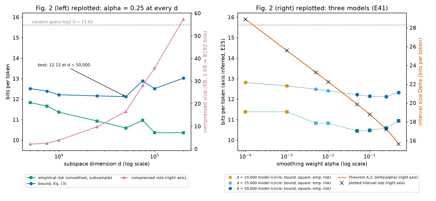
PAPER Fig. 2 and caption, p. 5; §4.3, p. 5 The left panel plots, against the subspace dimension \(d\), the empirical risk, the bound and the compressed size (in KB). The caption says \(d\) trades the degree of compression against the empirical risk and that \(d\) is optimized for the best bound. The right panel plots, against the smoothing weight \(\alpha\), the worst-case interval size \(\Delta\), the empirical risk and the bound. The caption says a different \(\alpha\) can be picked for each model after training; §4.3 says that as \(\alpha\) grows \(\Delta\) falls and the empirical risk rises, giving a sweet spot in the middle.

MY EXPLANATION Three earlier errata concern this figure: the right panel's bits-per-token axis has no tick labels (erratum E25), the left panel has eight values of \(d\) while Appendix E lists six (erratum E40), and the right panel combines three models (erratum E41, worked example (i)).

Worked example with real numbers¶

Everything in this section is MY EXPLANATION unless tagged. Numbers come from ch25_tables_audit.py (output sections in brackets). Its unstated inputs, used in every headline number below: \(\delta = 0.05\) SOURCE: authors' code, \(m\) = 8,009,762 documents and 8,823,811 sequences SOURCE: nanoGPT split / authors' code, 1 KB = 8,192 bits (erratum E35), \(V\) = 50,257 (erratum E36); \(n\) = 10,000 PAPER §6.1.

(a) The random-guess column¶

A model that assigns probability \(1/V\) to every token pays \(\log_2 V\) bits per token and misses the true token with probability \(1-k/V\) for top-k (Chapter 6). Output [1]:

Quantity	Exact	Paper
\(\log_2 V\) (bits/token)	15.6170	15.62
\(1-1/V\)	99.9980 %	99.99
\(1-10/V\)	99.9801 %	99.98
\(1-100/V\)	99.8010 %	99.80

Paper erratum E21: the top-1 random guess is truncated

PAPER Tables 1 and 4 The top-1 random-guess entry is 99.99. MY EXPLANATION \(1-1/V\) = 99.9980 %, which rounds to 100.00 at two decimals; the table truncates. The other three entries round correctly (output [1]). Table 2 mixes rounding conventions in the same way (erratum E46, logged by Chapter 6).

(b) Table 1 from Figure 1, and the 12.12¶

Chapter 23 showed that Figure 1 (left) contains every trained model as a point (training risk, complexity), and that the best point of each method reproduces Table 1. Output [2] repeats it:

Cell	training risk	+ complexity	= bound	Table 1
BPD, SubLoRA	10.5945	1.5278	12.1224	12.12
BPD, LoRA	11.4091	1.6856	13.0947	13.09
BPD, Subspace	13.8138	0.7758	14.5896	14.59
Top-1, SubLoRA	0.9148	0.0494	0.9641	96.41
Top-1, LoRA	0.9078	0.0980	1.0058	100 (capped)
Top-1, Subspace	0.9037	0.0616	0.9652	96.52

BPD entries are bits per token; top-1 entries are fractions (multiply by 100 for %). The top-10 and top-100 rows have no figure, so they cannot be checked.

Chapter 24 traced the best BPD model through Algorithm 1: compressed size 135,434.26 bits (16.5325 KB), smoothed subsampled empirical risk 10.5945 bits per token, \(\alpha = 0.25\). Eq. (3) gives 12.122180 bits per token, or 12.122225 with \(\log_2 576\) hyperparameter bits (output [2]). Both round to 12.12.

(c) Certified accuracy¶

An error bound of \(b\) says: with probability at least 0.95, the expected error is at most \(b\). Equivalently, the expected accuracy is at least \(1-b\). We call \(1-b\) the certified accuracy: the accuracy the bound guarantees.

Output [3], from Table 1:

	top-1	top-10	top-100
SubLoRA	3.59 %	22.10 %	41.66 %
Subspace	3.48 %	20.64 %	24.05 %
LoRA	0.00 %	15.63 %	32.74 %
uniform guesser, \(k/V\)	0.0020 %	0.0199 %	0.1990 %

SubLoRA's certified accuracy is 1,804, 1,111 and 209 times the uniform guesser's. So the guarantee is far from trivial in ratio terms, while small in absolute terms: the certified model gets the next token right at least 3.59 % of the time. Its measured training top-1 error is 0.9148, so its measured top-1 accuracy is 8.52 % (output [3]).

(d) Figure 2 (left), point by point¶

Figure 2 (left) gives, for each of eight values of \(d\), the compressed size, the empirical risk and the bound. All eight models use \(\alpha = 0.25\) (Chapter 16, its output [7]). So Eq. (3) can be recomputed from the first two and compared with the third.

It helps to factor the bound. With \(C\) the compressed size in bits, write

\[ K(C)=\sqrt{\frac{C\ln 2+2\ln C+\ln\frac{1}{s\delta}}{2m}}+\sqrt{\frac{\ln\frac{1}{(1-s)\delta}}{2n}}, \qquad s=\frac{n}{n+m}. \]

\(K(C)\) is a pure number: Eq. (3)'s two complexity terms divided by the interval width \(\Delta\). We call it the complexity factor. The BPD bound is "empirical risk \(+\ \Delta(\alpha)\,K(C)\)". A top-k bound is "empirical top-k error \(+\ K(C)\)", because there \(\Delta = 1\). (We use no hyperparameter bits here; Chapter 24 showed they move the bound by less than \(10^{-4}\).)

Output [4] (\(\Delta(0.25) = 17.2020\) bits per token):

\(d\)	size (KB)	bits per coordinate	\(K(C)\)	BPD cost \(17.202\,K\)	empirical risk	bound, Eq. (3)	plotted bound
5,000	2.1124	3.461	0.03964	0.6819	11.8332	12.5150	12.5156
7,500	2.5564	2.792	0.04237	0.7289	11.6587	12.3876	12.3881
10,000	3.8782	3.177	0.04934	0.8488	11.3655	12.2143	12.2147
25,000	9.8081	3.214	0.07122	1.2251	10.9345	12.1596	12.1599
50,000	16.5325	2.709	0.08881	1.5276	10.5945	12.1222	12.1224
75,000	27.9915	3.057	0.11186	1.9242	10.9667	12.8910	12.8911
100,000	35.7461	2.928	0.12481	2.1471	10.3626	12.5097	12.5098
200,000	57.3441	2.349	0.15482	2.6632	10.3638	13.0270	13.0271

Every recomputed bound matches the plotted one to within 0.0006 bits per token (the script asserts 0.003). Three observations:

The trade-off is real but shallow. Going from \(d\) = 5,000 to 50,000 lowers the empirical risk by 1.2386 bits per token and raises the BPD cost by 0.8458 (output [4]). The bound moves only from 12.5156 to 12.1224.
One point breaks the trend. At \(d\) = 75,000 the empirical risk is 10.967, higher than at 50,000 (10.595) and at 100,000 (10.363). The paper reports single runs, so this is presumably training noise or a different unreported setting (\(r\), learning rate, \(L_q\)). Without it the minimum might sit elsewhere; with it, \(d\) = 50,000 wins.
The models cost 2.35 to 3.46 bits per trained coordinate. That is below \(\log_2 17 = 4.087\), the most a code needs per coordinate with 17 quantization levels used equally often; for 11 levels the limit is \(\log_2 11 = 3.459\), which the \(d\) = 5,000 model just exceeds (codebook and counts add a fixed overhead, Chapter 22). Which \(L_q\) each model used is not reported (erratum E33).

PAPER §6.3, p. 7 The paper's point that a better validation loss is reachable: MY EXPLANATION the table shows it on the training side. The \(d\) = 100,000 and 200,000 models have empirical risk about 10.36, 0.2319 bits per token below the selected model (output [4]), yet worse bounds because they cost more.

(e) Which model made which cell¶

Each Table 1 cell is the best bound over all trained models for that row. Call this per-metric model selection. Because \(K(C)\) grows with \(C\), a cell's complexity pins down the compressed size of the model behind it: solve \(K(C) = \text{complexity}/\Delta\) for \(C\). We call the result the cell's implied compressed size. This is our analysis; the paper reports no compressed sizes for Table 1 (erratum E33).

Top-1 cells (\(\Delta = 1\), no \(\alpha\) needed; output [5]):

Method	complexity (Fig. 1)	implied size
SubLoRA	0.0494	3.883 KB
LoRA	0.0980	20.737 KB
Subspace	0.0616	6.865 KB

SubLoRA's 3.883 KB matches the \(d\) = 10,000 model of Figure 2 (left) (3.878 KB; \(K\) = 0.04934 against 0.04937 from Figure 1). So the SubLoRA top-1 cell (96.41) and the SubLoRA BPD cell (12.12) come from different models: about 3.9 KB and 16.5 KB. Which size wins a row depends on how fast the measured error falls as the model grows, compared with how fast the cost rises. For bits per token the 16.5 KB model wins; for top-1 a smaller one does. The paper gives no per-model top-1 errors, so we cannot say more about why. The observation fits the reading of the Figure 3 caption in which "smaller" means smaller compressed size (erratum E23, Chapter 26).

BPD cells need \(\Delta(\alpha)\), and the paper gives \(\alpha\) only for SubLoRA (0.25, Figure 2). Output [5] tries every \(\alpha\) of the grid:

\(\alpha\)	\(\Delta(\alpha)\)	SubLoRA (KB)	LoRA (KB)	Subspace (KB)
0.0001	28.905	4.649	5.984	0.596
0.001	25.581	6.355	8.115	0.918
0.005	23.254	8.058	10.234	1.253
0.01	22.246	8.980	11.380	1.440
0.05	19.865	11.793	14.869	2.023
0.1	18.787	13.458	16.931	2.376
0.25	17.202	16.537	20.737	3.040
0.5	15.617	20.661	25.828	3.948

SubLoRA at \(\alpha = 0.25\) gives 16.537 KB, the Figure 2 model (16.5325 KB). The method works.
LoRA at \(\alpha = 0.25\) gives 20.737 KB, exactly the size implied by LoRA's top-1 cell (difference 0.0003 KB). So, very likely, LoRA's best BPD model and best top-1 model are the same model, smoothed with \(\alpha = 0.25\). (Figure 1 has only four LoRA points.)
Subspace's top-1 model (6.865 KB) is larger than its BPD model at any \(\alpha\) (at most 3.948 KB): again two different models.

Top-10 and top-100 cells. No figure shows them. If the cell came from one of the eight Figure 2 models, its \(K\) lies between 0.0396 and 0.1548, so SubLoRA's empirical top-10 error was 0.624 to 0.739 and its top-100 error 0.429 to 0.544 (output [5]).

Paper erratum E66: the cells of one column come from different models

PAPER Table 1 caption, p. 6; Table 2 caption, p. 7 Table 1 reports the "best" bound per row; Table 2's caption makes the per-row choice explicit only for BPD. MY EXPLANATION The figures' own data show that the SubLoRA top-1 cell comes from a model of about 3.9 KB (\(d\) = 10,000) and the SubLoRA BPD cell from a 16.5 KB model (\(d\) = 50,000); likewise for Subspace. A reader who takes the column as the profile of one model is misled. Each cell is a valid statement about its own model; the column is not a statement about any single model. Impact: interpretation only.

(f) Table 2: units, perplexities and gaps¶

Output [6]:

	val BPD	× ln 2 (nats)	paper NLL	perplexity \(2^{\text{BPD}}\)	bound − val BPD	val − Fig. 1 smoothed train
SubLoRA	10.53	7.2988	7.29	1,478.6	1.59	−0.0645
LoRA	11.21	7.7702	7.77	2,368.9	1.88	−0.1991
Subspace	13.85	9.6001	9.60	14,766.1	0.74	+0.0362
Original	4.35	3.0152	3.01	20.4	66.41	—

Four readings.

"Validation NLL" is in nats per token. It equals BPD × ln 2 within 0.01 (erratum E27). SubLoRA's 7.29 is consistent with truncation, not rounding, of 7.2988 (erratum E46).
Perplexity puts the gap in plain terms. The certified SubLoRA model is, on validation text, as uncertain as a uniform choice among 1,478.6 tokens (in the geometric-mean sense of Chapter 6); the ordinary GPT-2 small, about 20. The bound itself, 12.12 bits, corresponds to 4,451.3; the uniform guesser to 50,257.
The bound − validation gap (1.59 bits per token for SubLoRA) is the distance between the guarantee and what was measured on held-out text. For the original model it is 66.41: the guarantee is useless there, although the model is the best.
Validation is below the smoothed training risk for SubLoRA and LoRA. A model normally does slightly worse on new data. Three effects can explain the reversal, and the paper does not say which apply (deeper block below): Table 2 may score the unsmoothed model, which removes a premium of up to \(\log_2(1/0.75) = 0.415\) bits per token at \(\alpha = 0.25\); it may average per token rather than per document (erratum E28); and the training risk is a 10,000-document estimate.

Paper errata E27, E28 and E47: what Table 2's validation rows measure

PAPER Table 2, p. 7 The table gives no unit for NLL and does not say which model or which average the validation rows use. [SOURCE: authors' code, estimate_loss, as recorded by Chapter 6] The released code tracks the validation loss of the unsmoothed model on random 1,024-token windows, a token-level average. MY EXPLANATION If Table 2 was produced that way, "bound 12.12 vs validation 10.53" compares a bound on the smoothed model's per-document average with the unsmoothed model's per-token average. The comparison is still informative about orders of magnitude, but not to the second decimal.

(g) The "Original Model" column¶

PAPER Table 1, p. 6; Table 2, p. 7; §6.2, p. 7 The ordinary GPT-2 small model gets a BPD bound of 70.76 (65.37 at the sequence level), top-k entries of 100, and validation BPD 4.35. The only description of how its bound was computed is §6.2's last sentence: quantization and arithmetic coding alone, without LoRA or a subspace.

Chapter 14 already reverse-engineered this entry (its output [6]); we re-print the key facts (output [7]):

"More than vacuous". A smoothed model's per-token loss is at most \(\log_2(V/\alpha)\): between 16.617 and 28.905 bits over the \(\alpha\) grid (Chapter 16). Both 70.76 and 65.37 exceed even the largest. The bound is above the worst loss the model could ever have.
What size it implies. Assume (our assumption, nothing in the paper) a smoothed training risk equal to the validation 4.35 bits per token. Then 70.76 corresponds to a code of 14.4 to 49.5 MiB (1 MiB = 8,388,608 bits), i.e. 0.98 to 3.36 bits per parameter for \(D\) = 123,689,472 parameters, depending on \(\alpha\). That is what quantizing to 11 or 17 levels and arithmetic-coding would give (at most \(\log_2 11 = 3.459\) or \(\log_2 17 = 4.087\) bits per parameter), consistent with §6.2's sentence. Chapter 14 found 13.7 to 50.1 MiB for assumed risks of 4 to 6 bits per token.
Why the top-k entries are 100. A top-k bound is at least \(K(C)\). \(K(C) \ge 1\) once \(C \ge\) 22,548,865 bits (2.69 MiB). Any model bigger than that gets a top-k bound of at least 100 %, whatever its training error. Raw float32 GPT-2 small has \(K\) = 13.10.

Paper erratum E67 (refines E53): the 'Original Model' bound is described in one sentence

PAPER §6.2, p. 7 Erratum E53 (logged by Chapter 14) says the method behind 70.76 is not stated. §6.2's closing sentence partly states it: quantization plus arithmetic coding of the full model. MY EXPLANATION This supports Chapter 14's third reading (a code of about 1 to 3.4 bits per parameter). Still missing: the number of levels, \(\alpha\), the empirical risk and whether the same Eq. (3) was used. The number remains unreproducible; only its qualitative message (vacuous) is solid.

(h) Table 4 against Table 1¶

PAPER Tables 1 and 4 Sequence-level minus document-level, cell by cell (percentage points; BPD in bits per token), from output [8]:

	SubLoRA	LoRA	Subspace	Original
Top-1	−0.24	+0.00	+0.88	+0.00
Top-10	+0.28	+1.48	+0.79	+0.00
Top-100	+0.38	−2.07	+0.16	+0.00
BPD	−0.03	−0.19	+0.09	−5.39

The paper attributes the differences to the empirical risk and a larger \(m\). How much can the larger \(m\) explain? If the same model with the same \(\alpha\) were used, only the \(m\)-term of Eq. (3) changes (the \(n\)-term changes by a relative \(1.9\times10^{-5}\)). The deeper block below proves that the drop is then at most the cell's complexity times \(1-\sqrt{m_{\text{doc}}/m_{\text{seq}}} = 0.0472\). Output [8]:

Cell	most the larger \(m\) can lower it	observed change
BPD, SubLoRA	0.072	−0.03
BPD, LoRA	0.080	−0.19
BPD, Subspace	0.037	+0.09
Top-1, SubLoRA	0.233 points	−0.24
Top-1, Subspace	0.291 points	+0.88
BPD, Original	3.343	−5.39

Seven of the twelve compressed-model cells rose, which a larger \(m\) alone can never cause. SubLoRA's top-1, LoRA's BPD and the Original's BPD fell by more than \(m\) can explain. So the empirical risk (or the selected model) differs between the tables, as Appendix B says.
For SubLoRA's BPD model the exact calculation gives an \(m\)-term of 1.3171 → 1.2548 and a bound of 12.1222 → 12.0600. Table 4 prints 12.09, so the sequence-level empirical risk was 0.025 to 0.035 bits per token higher (the range comes from the rounding of 12.09).
For the Original Model, keeping the assumed 4.35 and the implied size of (g) gives 67.63–67.64 at the sequence-level \(m\), not 65.37.

Paper erratum E54: the sequence-level bound is about the training corpus

PAPER §4.2, pp. 4–5; App. B, p. 14 The paper calls the two tables similar in value despite their different interpretation. MY EXPLANATION Chapter 15 proves that under the sequence-level reading the population is the training corpus, so Table 4 bounds training loss, not loss on new text. The closeness of the numbers does not make the statements alike. Chapter 15 also notes (a code note on the errata page, not a paper erratum) that the released code samples only 8,617 of the 8,823,811 chunks.

(i) Figure 2 (right) is an envelope¶

PAPER Fig. 2 right, p. 5 Read from the PDF, the plotted interval sizes agree with Theorem A.2's \(\Delta(\alpha) = \log_2\big(1+(1-\alpha)V/\alpha\big)\) to within 0.00006 bits per token at all eight \(\alpha\) (output [9]; the script asserts it).

Chapter 16 showed that the empirical-risk and bound curves are not one model's. For one model, \((\text{bound}-\text{empirical risk})/\Delta(\alpha) = K(C)\) does not depend on \(\alpha\). The plotted ratio takes three values (output [9]):

\(\alpha\)	\(K\)	implied size	model
0.0001, 0.001	0.0494	3.883 KB	\(d\) = 10,000
0.005, 0.01	0.0712	9.813 KB	\(d\) = 25,000
0.05, 0.1, 0.25, 0.5	0.0888	16.537 KB	\(d\) = 50,000

So each \(\alpha\) shows the best bound over several models. We call such a curve an envelope: the lower edge of a family of curves, here one per model. The same three models appear in both panels, which lets us follow each across \(\alpha\) (output [9]):

\(d\) = 50,000: empirical risk 10.453, 10.473, 10.595, 10.942 at \(\alpha\) = 0.05, 0.1, 0.25, 0.5 — it rises, as §4.3 says. Its bound is lowest, 12.1224, at \(\alpha = 0.25\).
\(d\) = 10,000: 11.385 (\(\alpha\) = 0.0001), 11.383 (0.001), 11.365 (0.25, left panel).
\(d\) = 25,000: 10.830 (0.005), 10.826 (0.01), 10.934 (0.25, left panel).

Paper erratum E41: Figure 2 (right) combines three models

PAPER Fig. 2 caption, p. 5 The caption presents the right panel as the effect of \(\alpha\). MY EXPLANATION It is an envelope over the \(d\) = 10,000, 25,000 and 50,000 models. The fall of the plotted empirical risk from 11.385 to 10.453 is mostly a change of model, not an effect of smoothing. Within the one model plotted at four values the risk only rises. No reported bound changes. The left axis of this panel has no tick labels (erratum E25); the values above use gridlines shared with the left panel, an inference that the \(\alpha = 0.25\) point confirms (it equals the left panel's best model).

Going deeper¶

This hub collects the derivations behind the chapter. Everything below is MY EXPLANATION unless tagged.

Going deeper: inverting Eq. (3) to recover a compressed size

What is fixed and what is random. Eq. (3) is a statement about the random draw of the \(m\) training documents and of the \(n\) subsample indices; the prior, \(\delta\), \(m\), \(n\) and \(\alpha\) are fixed in advance. Here we do no probability at all: we take published numbers and solve the bound's formula backwards. The result is a consistency check, not a new guarantee.

The factorization. Eq. (3) with the compression prior reads

\[ \text{bound}=\hat{\hat R}+\Delta\sqrt{\frac{\ln\frac1{P(h)}+\ln\frac1{s\delta}}{2m}} +\Delta\sqrt{\frac{\ln\frac1{(1-s)\delta}}{2n}}, \qquad \ln\frac1{P(h)}=C\ln2+2\ln C . \]

Here \(\hat{\hat R}\) is the subsampled empirical risk (bits per token for BPD, a fraction for top-k), \(\Delta\) the width of the loss interval in the same unit, \(C\) the compressed size in bits, and \(\ln\frac1{P(h)}\) the price in nats (Chapter 14). Both square roots are pure numbers, because their numerators are in nats (dimensionless) and their denominators are counts. Taking \(\Delta\) out:

\[ \text{bound}-\hat{\hat R}=\Delta\cdot K(C),\qquad K(C)=\sqrt{\frac{C\ln2+2\ln C+\ln\frac1{s\delta}}{2m}}+\sqrt{\frac{\ln\frac1{(1-s)\delta}}{2n}} . \]

Monotonicity. For \(C \ge 1\), \(\frac{d}{dC}(C\ln 2+2\ln C) = \ln 2 + 2/C > 0\), and the square root is increasing, so \(K\) is strictly increasing in \(C\). It starts at \(K(1) = 0.01305\) (output [4]), just above the \(n\)-term alone, and grows without limit. Hence for every target value \(k > K(1)\) there is exactly one \(C\) with \(K(C) = k\). The script finds it by a bracketing root-finder (brentq, which combines bisection with interpolation).

Using it. Figure 1 gives each point's complexity \(= \Delta K(C)\) in loss units. For top-k, \(\Delta = 1\) and \(C = K^{-1}(\text{complexity})\) directly. For BPD, \(\Delta = \Delta(\alpha)\) and \(C = K^{-1}(\text{complexity}/ \Delta(\alpha))\), one candidate per \(\alpha\). Larger \(\Delta\) (smaller \(\alpha\)) means a smaller implied \(C\), which is the pattern in the table of worked example (e).

Error budget. The figure coordinates are exact to about \(10^{-4}\) (they reproduce Table 1 and the 12.12). Differentiating the first square root \(K_m\) (the second does not depend on \(C\)): \(dK/dC = (\ln 2 + 2/C)/(4mK_m) \approx (\ln 2)/(4mK_m)\) per bit for \(C\) of \(10^5\) bits. Near 16.5 KB this is \(2.826\times10^{-7}\) per bit, so a change of \(10^{-4}\) in \(K\) moves \(C\) by 354 bits, about 0.04 KB (output [4]), consistent with 16.537 vs 16.5325 KB. What the inversion cannot see: hyperparameter bits (9.17 bits, invisible at this precision) and whether \(\delta\), \(m\) and the KB convention are the ones we assumed. Their agreement with Figure 2's printed sizes is the evidence that they are.

Going deeper: why top-k bounds need no smoothing and no choice of α

Claim. The top-k error of the smoothed model \(p_h = (1-\alpha)p_\theta + \alpha/V\) equals that of the base model \(p_\theta\), for every \(\alpha\in(0,1)\).

Proof. Fix a context \(x_{<i}\). For two tokens \(a, b\), \(p_h(a) - p_h(b) = (1-\alpha)\big(p_\theta(a) - p_\theta(b)\big)\), because the \(\alpha/V\) terms cancel. Since \(1-\alpha>0\), \(p_h(a) > p_h(b)\) exactly when \(p_\theta(a) > p_\theta(b)\). So the two models order all tokens the same way, their top-k sets coincide (with the same tie-breaking rule), and the indicator \(\mathbf 1[x_i \notin \mathrm{Top}_k]\) is the same for both. Averaging over tokens and documents preserves the equality. \(\square\) (Chapter 16 checks this numerically.)

Consequences. (1) The top-k loss is in \([0,1]\) for any model, so \(\Delta = 1\) without smoothing. (2) A top-k cell certifies the quantized model itself, not a smoothed variant: its bound is about the model one would actually run. (3) Since \(\alpha\) plays no role, the top-1 cells' complexities pin down \(C\) with no unknown, which is why worked example (e) can identify the 3.883 KB model.

Going deeper: how much a larger m can lower a bound

Setting. Same model (so same price \(A = \ln\frac1{P(h)}\) in nats), same \(\alpha\) (so same \(\Delta\)), same \(n\). Only \(m\) changes, from \(m\) to \(m' > m\), so \(s = n/(n+m)\) becomes \(s' = n/(n+m') < s\).

The \(m\)-term. \(T_m = \Delta\sqrt{(A + \ln\frac1{s\delta})/(2m)}\). Because \(s' < s\), \(\ln\frac1{s'\delta} > \ln\frac1{s\delta}\), so

\[ T_m' = \Delta\sqrt{\frac{A+\ln\frac1{s'\delta}}{2m'}} \ \ge\ \Delta\sqrt{\frac{A+\ln\frac1{s\delta}}{2m'}} = T_m\sqrt{\frac{m}{m'}} . \]

Hence the drop is \(T_m - T_m' \le T_m\big(1-\sqrt{m/m'}\big)\).

The \(n\)-term. \(T_n = \Delta\sqrt{\ln\frac1{(1-s)\delta}/(2n)}\). With \(s' < s\), \(1-s' > 1-s\), so \(T_n\) also falls, but only by a relative \(1-\sqrt{\ln\frac1{(1-s')\delta}\big/\ln\frac1{(1-s)\delta}} = 1.9\times10^{-5}\) (output [8]): at most \(4\times10^{-6}\) bits per token for \(T_n \approx 0.21\).

Putting it together. The complexity shown in Figure 1 is \(T_m + T_n \ge T_m\). So the total drop is at most \((T_m+T_n)(1-\sqrt{m/m'})\) up to the negligible \(n\)-term change. With \(m\) = 8,009,762 and \(m'\) = 8,823,811 SOURCE: authors' code, \(1-\sqrt{m/m'} = 0.0472\). For the Original Model, whose complexity we do not know, the complexity is at most \(70.76 - \hat{\hat R} \le 70.76\), because a smoothed loss is positive. This gives the cap 3.343 in worked example (h). Any observed change beyond the cap, or in the other direction, must come from the empirical risk or from a different selected model.

Going deeper: what a whole table certifies

One cell. Theorem A.1 with the subsampling step (Eq. 3) says: with probability at least \(1-\delta\) over the draw of the training documents and of the subsample, \(R(\hat h) \le \text{bound}(\hat h)\) — simultaneously for all hypotheses in the prior's support, through the prior-weighted union bound (Chapter 11), up to the selection caveat of erratum E07. One cell is one such statement, for one loss.

Several losses. The top-1, top-10, top-100 and BPD statements use different losses, so they are different theorems, each with its own failure event \(B_j\) of probability at most \(\delta\). The probability that all four hold is

\[ \Pr\Big[\bigcap_{j=1}^{4} B_j^{c}\Big] = 1-\Pr\Big[\bigcup_{j=1}^{4}B_j\Big] \ \ge\ 1-\sum_{j=1}^{4}\Pr[B_j] \ \ge\ 1-4\delta = 0.80, \]

by the union bound (Chapter 10); for all twelve compressed-model cells, \(1-12\delta = 0.40\) (output [10]). These are worst-case guarantees; the true joint probability is probably higher because the events are positively related (they share the data), but the theorems do not show it. To make a whole column hold at 95 % jointly, run each loss at \(\delta/4\): this adds \(\ln 4\) nats inside the \(m\)-term and inside the \(n\)-term, a tiny change for the \(m\)-term (whose price is about \(9.4\times10^4\) nats) but a visible one for the \(n\)-term. For the best BPD model the \(n\)-term grows from 0.2106 to 0.2547 and the bound from 12.1222 to 12.1663 bits per token (output [10]).

Choosing among methods. Reading off the best column (bold) is another selection. It can be paid for by giving each method prior weight 1/3: \(\log_2 3 = 1.585\) extra bits, which moves the BPD bound by \(+7.7\times10^{-6}\) (output [10]). The paper does not mention it; it does not matter numerically.

Going deeper: how validation can come out below training

Write \(\ell_\theta\) for the per-token loss \(-\log_2 p_\theta(x_i\mid x_{<i})\) of the base model and \(\ell_h\) for that of the smoothed model with weight \(\alpha\).

Smoothing can raise the loss of well-predicted tokens, by a bounded amount. Since \(p_h \ge (1-\alpha)p_\theta\),

\[ \ell_h = -\log_2 p_h \le -\log_2\big((1-\alpha)p_\theta\big) = \ell_\theta + \log_2\frac1{1-\alpha}, \]

which is \(\ell_\theta + 0.415\) bits at \(\alpha = 0.25\). Smoothing lowers the loss of tokens with \(p_\theta < 1/V\) (Chapter 16). So the smoothed training risk can sit anywhere from somewhat below to at most 0.415 bits above the unsmoothed one.

Three sources of the observed \(-0.0645\) (SubLoRA) and \(-0.1991\) (LoRA).

Different model: if validation scores \(p_\theta\) and training scores \(p_h\), a premium of up to 0.415 bits separates them.
Different average: a per-token average weights long documents more; Chapter 6 shows the two averages differ by \(\mathrm{Cov}(L,\text{BPD})/\bar L\), which can have either sign.
Noise: the training value is a 10,000-document estimate. Its Hoeffding half-width at 95 % is the \(n\)-term, 0.21 bits per token (Chapter 24), so differences of 0.06 to 0.2 are within the noise the bound itself allows.

None of these can be separated with the published numbers. The point for the reader: the "generalization gap" of these models is too small to measure from the tables. They are so constrained that they do not overfit; the bound's 1.59 bits come from the price of guaranteeing it, not from a measured gap.

Common misconceptions¶

Misconception: The SubLoRA column of Table 1 describes one model with top-1 error at most 96.41 % and at most 12.12 bits per token. — Actually: each cell is the best bound for its own row. The top-1 cell comes from a model of about 3.9 KB (\(d\) = 10,000), the BPD cell from a 16.5 KB model (\(d\) = 50,000) (worked example (e)).
Misconception: A top-1 error bound of 96.41 % means the model is wrong 96.41 % of the time. — Actually: it is an upper bound on the expected error, holding with probability at least 0.95. The model's measured training error is 91.48 %. The certified accuracy, 3.59 %, is 1,804 times the uniform guesser's.
Misconception: The original model's 70.76 shows that it generalizes badly. — Actually: it has the best validation loss in Table 2 (4.35 bits per token). 70.76 exceeds the largest loss any smoothed model can have; it says only that this guarantee method fails for a model that large.
Misconception: Validation 10.53 vs bound 12.12 shows the bound is tight to within 1.59 bits for a good language model. — Actually: the certified model has perplexity 1,478.6 against GPT-2 small's 20.4, and the two numbers may measure different models (smoothed vs not) and different averages (errata E27, E28).
Misconception: Table 4 confirms Table 1 at the sequence level. — Actually: Table 4 bounds the loss on the training corpus itself (Chapter 15); the near-equality of the numbers does not make the two statements comparable.
Misconception: Figure 2 (right) shows how one model's empirical risk changes with \(\alpha\). — Actually: it is an envelope over three models (erratum E41). Within one model the empirical risk rises with \(\alpha\).

Self-test¶

Q1. The \(d\) = 25,000 model of Figure 2 has complexity factor \(K\) = 0.07122. Suppose its empirical top-1 error on the subsample were 0.92. What top-1 error bound and what certified top-1 accuracy would it get? Would it beat SubLoRA's Table 1 entry?

Answer

A top-1 bound has \(\Delta = 1\), so bound \(= 0.92 + 0.07122 = 0.99122\), i.e. 99.12 %, and the certified accuracy is 0.88 % (output [Q1]). It does not beat 96.41 %. It is non-vacuous (below 99.998 %), but barely: the model would need a measured error below \(0.99998 - 0.07122\) to be non-vacuous at all, and much lower to compete.

Q2. A colleague writes: "the paper's best model, 16.5 KB, has top-1 error at most 96.41 %". What is wrong, and what would you need to state the 16.5 KB model's top-1 bound?

Answer

The 96.41 % cell comes from a different model: its complexity 0.0494 implies 3.883 KB, the \(d\) = 10,000 model (worked example (e)). For the 16.5 KB model the top-1 complexity would be \(K\) = 0.08881 (output [4]), so its bound is its empirical top-1 error plus 0.08881. The paper does not report that empirical error, so its top-1 bound cannot be stated from the paper.

Q3. Table 4's SubLoRA BPD bound is 12.09, 0.03 below Table 1's 12.12. If the very same 16.5 KB model, with the same empirical risk, were evaluated with the sequence-level \(m\) = 8,823,811 SOURCE: authors' code, what would the bound be? What does the comparison imply?

Answer

Only the \(m\)-term changes: 1.3171 → 1.2548, so the bound becomes 12.0600 (output [8]). Table 4 prints 12.09, so the sequence-level empirical risk must have been 0.025 to 0.035 bits per token higher than the document-level one, which matches Appendix B's statement that the empirical risk evaluation differs. In any case the two numbers certify different things: new documents (Table 1) versus the training corpus (Table 4, Chapter 15).

Code for this chapter¶

Run it from the project root:

.venv/Scripts/python explainer/code/ch25_tables_audit.py

Source: ch25_tables_audit.py

"""Chapter 25 demo: auditing the GPT-2-small results of arXiv 2312.17173 (Tables 1, 2, 4 and Figure 2).

Claims reproduced / checked (paper values typed in from the PDF; figure data read by fig_extract.py):
  [1] Random-guess column of Tables 1 and 4: log2 V = 15.62 and 1 - k/V for k = 1, 10, 100 (erratum E21).
  [2] Table 1's BPD and Top-1 cells for SubLoRA / LoRA / Subspace from Figure 1's exact points (as in Ch. 23),
      and the Eq. (3) value 12.12 for the best model (as in Ch. 24).
  [3] Certified accuracies 1 - bound (SubLoRA: 3.59 %, 22.10 %, 41.66 %) vs the uniform guesser.
  [4] Figure 2 (left): Eq. (3) recomputed from each plotted (compressed size, empirical risk) at alpha = 0.25
      reproduces each plotted bound; the per-unit-width complexity K(C) of each model.
  [5] Implied compressed sizes of Table 1's best points (MY ANALYSIS): top-1 (width 1) and BPD (width Delta(alpha)).
  [6] Table 2: Validation NLL = BPD x ln 2 (nats, E27), perplexities, bound - validation gaps.
  [7] "Original Model" 70.76: above log2(V/alpha) for every alpha; size implied under assumptions; top-k = 100.
  [8] Table 4 vs Table 1 cell by cell; the most that the larger sequence-level m can explain.
  [9] Figure 2 (right): interval curve = Theorem A.2's Delta(alpha); three models (erratum E41, Ch. 16).
 [10] Joint confidence of a whole table column (union bound).
Assumptions not stated in the paper (labelled in the output): delta = 0.05, m = 8,009,762 documents,
m = 8,823,811 sequences [SOURCE: authors' code / nanoGPT]; 1 KB = 8192 bits (E35); V = 50,257.
Writes outputs/ch25_tables_audit.txt and docs/assets/fig/ch25_fig2_replot.png.
"""
from __future__ import annotations

import json
import math
import subprocess
import sys
import time
from pathlib import Path

HERE = Path(__file__).resolve().parent
sys.path.insert(0, str(HERE))
import pacbound as pb  # noqa: E402

import numpy as np  # noqa: E402
from scipy.optimize import brentq  # noqa: E402
import matplotlib  # noqa: E402

matplotlib.use("Agg")
import matplotlib.pyplot as plt  # noqa: E402

T0 = time.time()
JSON = HERE / "outputs" / "fig_extract.json"
OUT_TXT = HERE / "outputs" / "ch25_tables_audit.txt"
FIG = HERE.parent / "docs" / "assets" / "fig" / "ch25_fig2_replot.png"
if not JSON.exists():
    subprocess.run([sys.executable, str(HERE / "fig_extract.py")], check=True)
DATA = json.loads(JSON.read_text(encoding="utf-8"))

lines: list[str] = []


def out(s: str = "") -> None:
    print(s)
    lines.append(s)


V, M, MS, N, DEL = pb.V_GPT2, pb.M_DOCS, pb.M_SEQS, pb.N_SUB, pb.DELTA
KB = 8192.0                      # bits per KB [SOURCE: Lotfi et al. 2022; erratum E35]
MIB = 8 * 1024 * 1024            # bits per MiB
LOG2V = pb.random_guess_bpd(V)
D_SMALL = pb.gpt2_params(12, 768)
ALPHAS = pb.ALPHA_GRID
METH = ["SubLoRA", "LoRA", "Subspace"]

# ---- Paper values [PAPER Table 1 p. 6, Table 2 p. 7, Table 4 p. 14] (percent for top-k, bits/token for BPD)
COLS = ["SubLoRA", "LoRA", "Subspace", "Original", "Random"]
ROWS = ["Top-1", "Top-10", "Top-100", "BPD"]
T1 = {"Top-1": [96.41, 100, 96.52, 100, 99.99], "Top-10": [77.90, 84.37, 79.36, 100, 99.98],
      "Top-100": [58.34, 67.26, 75.95, 100, 99.80], "BPD": [12.12, 13.09, 14.59, 70.76, 15.62]}
T4 = {"Top-1": [96.17, 100, 97.40, 100, 99.99], "Top-10": [78.18, 85.85, 80.15, 100, 99.98],
      "Top-100": [58.72, 65.19, 76.11, 100, 99.80], "BPD": [12.09, 12.90, 14.68, 65.37, 15.62]}
T2_VAL_BPD = [10.53, 11.21, 13.85, 4.35]
T2_VAL_NLL = [7.29, 7.77, 9.60, 3.01]


def price(c_bits: float, extra: float = 0.0) -> float:
    """ln 1/P(h) in nats for a C-bit model (paper §4.1 form, via pacbound)."""
    return pb.log_inv_prior_nats_from_bits(c_bits, extra)


def K_of(c_bits: float, m: int = M, extra: float = 0.0) -> float:
    """Eq. (3) complexity per unit width, (term_m + term_n)/Delta, for a C-bit model. Dimensionless."""
    t1, t2 = pb.eq3_terms(price(c_bits, extra), m, N, DEL, width=1.0)
    return t1 + t2


def C_of_K(k: float, m: int = M) -> float:
    """Invert K_of: compressed size (bits) whose Eq. (3) complexity per unit width equals k."""
    return brentq(lambda c: K_of(c, m) - k, 2.0, 1e12, xtol=1e-6, rtol=1e-12)


def delta_a(a: float) -> float:
    """Theorem A.2 width Delta(alpha) in bits/token (pacbound)."""
    return pb.smoothing_interval(a, V)[2]


# =============================================================================================
out(f"Chapter 25 - GPT-2-small results audit (ch25_tables_audit.py). [0] V = {V:,}; m = {M:,} docs / {MS:,} seqs, delta = {DEL} [SOURCE: authors' code/nanoGPT]; "
    f"n = {N:,}; 1 KB = 8192 bits (E35)")

# [1] random-guess column -------------------------------------------------------------------
rg = [100 * pb.random_guess_topk_error(k, V) for k in (1, 10, 100)]
out(f"[1] Random guess: BPD log2 V = {LOG2V:.4f} (paper 15.62); top-1 {rg[0]:.4f} % (paper 99.99 = truncated; "
    f"rounds to {round(rg[0], 2):.2f}, E21); top-10 {rg[1]:.4f} % (99.98); top-100 {rg[2]:.4f} % (99.80)")
assert abs(LOG2V - 15.62) < 0.005 and math.floor(rg[0] * 100) / 100 == 99.99
assert abs(rg[1] - 99.98) < 0.005 and abs(rg[2] - 99.80) < 0.005

# [2] Table 1 from Figure 1 -------------------------------------------------------------------
out("[2] Table 1 from Figure 1's exact points (best = min of train + complexity; as in Ch. 23)")
F1 = DATA["figure1"]
best = {}
for panel, row in (("left_bpd", "BPD"), ("left_top1", "Top-1")):
    parts = []
    for j, meth in enumerate(METH):
        p = min(F1[panel]["points"][meth], key=lambda q: q["sum"])
        best[(row, meth)] = p
        rep = p["sum"] if row == "BPD" else min(100 * p["sum"], 100.0)
        assert abs(rep - T1[row][j]) < 0.005 + 1e-9
        parts.append(f"{meth} {p['train_risk']:.4f}+{p['complexity']:.4f}={p['sum']:.4f}"
                     + (" (>1: printed as 100)" if row == "Top-1" and p["sum"] > 1 else ""))
    out(f"  {row:5s}: " + "; ".join(parts))
C_BEST = DATA["figure2"]["left"]["compressed_size_kb"][4]["value"] * KB
EMP_BEST = DATA["figure2"]["left"]["empirical_risk"][4]["value"]
b0 = pb.eq3_bound(EMP_BEST, price(C_BEST), M, N, DEL, width=delta_a(0.25))
b576 = pb.eq3_bound(EMP_BEST, price(C_BEST, math.log2(576)), M, N, DEL, width=delta_a(0.25))
out(f"  Eq. (3), best model (C = {C_BEST:,.2f} bits = {C_BEST / KB:.4f} KB, alpha 0.25): {b0:.6f} "
    f"(+log2 576 bits: {b576:.6f}); paper 12.12 (Ch. 24)")
assert abs(round(b0, 2) - 12.12) < 1e-9 and abs(C_BEST - 135434.26) < 0.01

# [3] certified accuracies --------------------------------------------------------------------
out("[3] Certified accuracy = 100 % - error bound (Table 1), top-1 / top-10 / top-100")
acc = {meth: [100 - T1[r][j] for r in ("Top-1", "Top-10", "Top-100")] for j, meth in enumerate(METH)}
out("  " + "; ".join(f"{m_}: {a[0]:.2f} / {a[1]:.2f} / {a[2]:.2f} %" for m_, a in acc.items()))
uni = [100 * k / V for k in (1, 10, 100)]
out(f"  uniform guesser k/V: {uni[0]:.4f} / {uni[1]:.4f} / {uni[2]:.4f} %;  SubLoRA / uniform: "
    + " / ".join(f"{a / u:,.0f}x" for a, u in zip(acc["SubLoRA"], uni))
    + f"; SubLoRA top-1 model's training accuracy 1 - {best[('Top-1', 'SubLoRA')]['train_risk']:.4f} = "
    f"{100 * (1 - best[('Top-1', 'SubLoRA')]['train_risk']):.2f} %")

# [4] Figure 2 left ---------------------------------------------------------------------------
out("[4] Fig. 2 (left): Eq. (3) at alpha = 0.25 from plotted size + empirical risk, vs plotted bound")
out("        d   C (KB)  bits/coord  K (=top-k cost)  BPD cost  emp risk  bound(Eq.3)  plotted    diff")
F2L = DATA["figure2"]["left"]
DL = [int(round(p["d"], -2)) for p in F2L["bound"]]
CKB = [p["value"] for p in F2L["compressed_size_kb"]]
EMPL = [p["value"] for p in F2L["empirical_risk"]]
BNDL = [p["value"] for p in F2L["bound"]]
KL = []
for d, ck, e, bp in zip(DL, CKB, EMPL, BNDL):
    k = K_of(ck * KB)
    KL.append(k)
    bb = e + delta_a(0.25) * k
    out(f"  {d:7,d}  {ck:7.4f}  {ck * KB / d:9.3f}  {k:14.5f}  {delta_a(0.25) * k:8.4f}  {e:8.4f}  "
        f"{bb:10.4f}  {bp:8.4f}  {bb - bp:+.4f}")
    assert abs(bb - bp) < 0.003
i_min = int(np.argmin(BNDL))
out(f"  min plotted bound {BNDL[i_min]:.4f} at d = {DL[i_min]:,}; d = 75,000 breaks the trend (emp {EMPL[5]:.3f} "
    f"vs {EMPL[4]:.3f} at 50k, {EMPL[6]:.3f} at 100k); log2 11 = {math.log2(11):.3f}, log2 17 = {math.log2(17):.3f}")
out(f"  5k -> 50k: emp {EMPL[4] - EMPL[0]:+.4f}, BPD cost {delta_a(0.25) * (KL[4] - KL[0]):+.4f}; 100k emp "
    f"{EMPL[6] - EMPL[4]:+.4f} vs 50k; n-term alone (C -> 1) K = {K_of(1.0):.5f}; at 16.5 KB dK/dC = "
    f"{(K_of(C_BEST + 1) - K_of(C_BEST - 1)) / 2:.3e} per bit -> dK 1e-4 = {1e-4 / ((K_of(C_BEST + 1) - K_of(C_BEST - 1)) / 2):.0f} bits")

# [5] implied compressed sizes ------------------------------------------------------------------
ctop = {meth: C_of_K(best[("Top-1", meth)]["complexity"]) / KB for meth in METH}
out("[5] Implied C [MY ANALYSIS; Eq. (3), no hyperparameter bits]. Top-1 (width 1): "
    + "; ".join(f"{m_} {ctop[m_]:.3f} KB" for m_ in METH))
out(f"  SubLoRA top-1 = Fig. 2 d = 10,000 model ({CKB[2]:.3f} KB, K {KL[2]:.5f} vs "
    f"{best[('Top-1', 'SubLoRA')]['complexity']:.5f}); its empirical top-1 error "
    f"{best[('Top-1', 'SubLoRA')]['train_risk']:.4f}")
out("  BPD (width Delta(alpha); alpha unstated except SubLoRA's 0.25), implied C in KB:")
out("     alpha   Delta   SubLoRA     LoRA  Subspace")
cbpd = {}
for a in ALPHAS:
    w = delta_a(a)
    cbpd[a] = [C_of_K(best[("BPD", meth)]["complexity"] / w) / KB for meth in METH]
    out(f"    {a:6g}  {w:6.3f}  {cbpd[a][0]:8.3f} {cbpd[a][1]:8.3f} {cbpd[a][2]:8.3f}")
assert abs(cbpd[0.25][0] - 16.5325) < 0.01 and abs(cbpd[0.25][1] - ctop["LoRA"]) < 0.01
out(f"  LoRA: BPD point at alpha 0.25 ({cbpd[0.25][1]:.3f} KB) = its top-1 point ({ctop['LoRA']:.3f} KB, "
    f"diff {cbpd[0.25][1] - ctop['LoRA']:+.4f}); "
    f"Subspace top-1 {ctop['Subspace']:.3f} KB > its BPD C at every alpha (max {max(c[2] for c in cbpd.values()):.3f})")
kmin, kmax = min(KL), max(KL)
out(f"  top-k cost K of the 8 Fig. 2 models {kmin:.4f}..{kmax:.4f} -> if one of them made the cell: empirical "
    f"top-10 error {0.7790 - kmax:.3f}..{0.7790 - kmin:.3f}, top-100 {0.5834 - kmax:.3f}..{0.5834 - kmin:.3f}")

# [6] Table 2 ---------------------------------------------------------------------------------
out("[6] Table 2: NLL = BPD x ln 2 (nats/token, E27); perplexity 2^BPD; bound - validation (bits/token)")
for j, meth in enumerate(METH + ["Original"]):
    b, nll = T2_VAL_BPD[j], T2_VAL_NLL[j]
    tr = ""
    if meth != "Original":
        t = best[("BPD", meth)]["train_risk"]
        tr = f"; Fig. 1 smoothed train {t:.4f} (val - train {b - t:+.4f})"
    out(f"  {meth:8s} val {b:5.2f} x ln2 = {b * pb.LN2:.4f} (paper {nll:.2f}); ppl {2 ** b:8,.1f}; "
        f"gap {T1['BPD'][j] - b:5.2f}{tr}")
    assert abs(b * pb.LN2 - nll) < 0.01
out(f"  ppl at the bound 2^12.12 = {2 ** 12.12:,.1f}; uniform 2^log2V = {2 ** LOG2V:,.0f}; "
    f"smoothing premium cap at alpha 0.25: log2(1/0.75) = {math.log2(1 / 0.75):.3f} bits/token")

# [7] Original Model --------------------------------------------------------------------------
his = [math.log2(V / a) for a in ALPHAS]
out(f"[7] 'Original Model' 70.76 / 65.37: max smoothed loss log2(V/alpha) over the grid {min(his):.3f}.."
    f"{max(his):.3f} < both -> 'more than vacuous' (Ch. 14)")
assert max(his) < 65.37
RH = 4.35  # ASSUMPTION: smoothed training risk = Table 2's validation BPD
cs, preds = [], []
for a in ALPHAS:
    w = delta_a(a)
    c = brentq(lambda c: pb.eq3_bound(RH, price(c), M, N, DEL, width=w) - 70.76, 1e3, 1e12, rtol=1e-12)
    cs.append(c)
    preds.append(pb.eq3_bound(RH, price(c), MS, N, DEL, width=w))
out(f"  ASSUMED emp risk {RH}: implied C {min(cs) / MIB:.1f}..{max(cs) / MIB:.1f} MiB = "
    f"{min(cs) / D_SMALL:.2f}..{max(cs) / D_SMALL:.2f} bits/param (D = {D_SMALL:,}) over the alpha grid")
out(f"  same C and emp risk at m = {MS:,}: bound {min(preds):.2f}..{max(preds):.2f} vs Table 4's 65.37")
c_vac = C_of_K(1.0)
out(f"  top-k bound >= 100 % whatever the training error once K(C) >= 1, i.e. C >= {c_vac:,.0f} bits = "
    f"{c_vac / MIB:.2f} MiB; float32 GPT-2 small: K = {K_of(32.0 * D_SMALL):.2f}")

# [8] Table 4 vs Table 1 ----------------------------------------------------------------------
out("[8] Table 4 (sequence level) minus Table 1 (document level), cell by cell (pct pts; BPD in bits/token)")
for r in ROWS:
    out(f"  {r:7s} " + "  ".join(f"{c} {T4[r][j] - T1[r][j]:+6.2f}" for j, c in enumerate(COLS[:4])))
shrink = 1 - math.sqrt(M / MS)
caps = []
for (r, meth) in (("BPD", "SubLoRA"), ("BPD", "LoRA"), ("BPD", "Subspace"), ("Top-1", "SubLoRA"),
                  ("Top-1", "Subspace")):
    j = COLS.index(meth)
    cap = best[(r, meth)]["complexity"] * (100 if r == "Top-1" else 1) * shrink
    caps.append(f"{r} {meth} {cap:.3f} (obs. {T4[r][j] - T1[r][j]:+.2f})")
out(f"  max drop from larger m = complexity x (1 - sqrt(m_doc/m_seq)) = complexity x {shrink:.4f}: " + "; ".join(caps[:2]))
out("    " + "; ".join(caps[2:]) + f"; BPD Original {70.76 * shrink:.3f} (obs. {65.37 - 70.76:+.2f})")
s_d, s_s = N / (N + M), N / (N + MS)
nfac = 1 - math.sqrt(math.log(1 / ((1 - s_s) * DEL)) / math.log(1 / ((1 - s_d) * DEL)))
tm_d, _ = pb.eq3_terms(price(C_BEST), M, N, DEL, width=delta_a(0.25))
tm_s, _ = pb.eq3_terms(price(C_BEST), MS, N, DEL, width=delta_a(0.25))
b_seq = pb.eq3_bound(EMP_BEST, price(C_BEST), MS, N, DEL, width=delta_a(0.25))
out(f"  exact, best BPD model: m-term {tm_d:.4f} -> {tm_s:.4f}, bound {b0:.4f} -> {b_seq:.4f}; Table 4 12.09 "
    f"-> seq-level emp risk {12.085 - b_seq:+.3f}..{12.095 - b_seq:+.3f}; n-term shrinks by a factor {nfac:.1e}")

# [9] Figure 2 right --------------------------------------------------------------------------
F2R = DATA["figure2"]["right"]
WR = [p["value"] for p in F2R["worst_case_interval"]]
ER = [p["value"] for p in F2R["empirical_risk"]]
BR = [p["value"] for p in F2R["bound"]]
dmax = max(abs(w - delta_a(a)) for w, a in zip(WR, ALPHAS))
assert dmax < 5e-4
KR = [(b - e) / delta_a(a) for b, e, a in zip(BR, ER, ALPHAS)]
groups: dict[float, list] = {}
for a, k in zip(ALPHAS, KR):
    groups.setdefault(round(k, 4), []).append((a, k))
out(f"[9] Fig. 2 (right): max |plotted interval - Delta(alpha)| = {dmax:.5f} bits/token; K = (bound - emp)/Delta:")
out("  " + "; ".join(f"{np.mean([k for _, k in g]):.4f} at alpha {','.join(f'{a:g}' for a, _ in g)} -> "
                     f"{C_of_K(float(np.mean([k for _, k in g]))) / KB:.3f} KB" for g in groups.values()))
out(f"  d = 50k model, emp risk at alpha 0.05/0.1/0.25/0.5: " + ", ".join(f"{e:.3f}" for e in ER[4:])
    + f" (rises); bound minimum {min(BR):.4f} at alpha {ALPHAS[int(np.argmin(BR))]}")
out(f"  same model in both panels: d = 10k emp {ER[0]:.3f} (alpha 1e-4), {ER[1]:.3f} (1e-3), {EMPL[2]:.3f} (0.25); "
    f"d = 25k {ER[2]:.3f} (0.005), {ER[3]:.3f} (0.01), {EMPL[3]:.3f} (0.25)")

# [10] joint confidence -----------------------------------------------------------------------
out(f"[10] Union bound: 4 cells of a column all hold w.p. >= {1 - 4 * DEL:.2f}, 12 compressed-model cells >= "
    f"{1 - 12 * DEL:.2f}; picking the best of 3 methods via the prior: log2 3 = {math.log2(3):.3f} bits -> BPD "
    f"bound {pb.eq3_bound(EMP_BEST, price(C_BEST, math.log2(3)), M, N, DEL, width=delta_a(0.25)) - b0:+.1e}; "
    f"best BPD model at delta/4: {pb.eq3_bound(EMP_BEST, price(C_BEST), M, N, DEL / 4, width=delta_a(0.25)):.4f} "
    f"(n-term {pb.eq3_terms(price(C_BEST), M, N, DEL / 4, width=delta_a(0.25))[1]:.4f})")
out(f"[Q1] d = 25,000 model (K {KL[3]:.5f}), empirical top-1 error 0.92: bound {0.92 + KL[3]:.5f} = "
    f"{100 * (0.92 + KL[3]):.2f} %, certified top-1 accuracy {100 * (1 - 0.92 - KL[3]):.2f} %")

# ---- figure --------------------------------------------------------------------------------
plt.rcParams.update({"font.size": 11})
fig, (ax1, ax2) = plt.subplots(1, 2, figsize=(13, 6.0))
ax1.plot(DL, EMPL, "s-", color="#009E73", label="empirical risk (smoothed, subsample)")
ax1.plot(DL, BNDL, "o-", color="#0072B2", label="bound, Eq. (3)")
ax1.axhline(LOG2V, ls="--", color="grey", lw=1)
ax1.text(5200, LOG2V + 0.08, "random guess log2 V = 15.62", color="grey", fontsize=9)
ax1.annotate("best: 12.12 at d = 50,000", (DL[i_min], BNDL[i_min]), xytext=(6000, 13.6),
             arrowprops=dict(arrowstyle="->", color="black"), fontsize=9)
ax1.set_xscale("log")
ax1.set_xlabel("subspace dimension d (log scale)")
ax1.set_ylabel("bits per token")
ax1.set_ylim(9.5, 16.2)
ax1b = ax1.twinx()
ax1b.plot(DL, CKB, "^-", color="#CC79A7", label="compressed size (right axis)")
ax1b.set_ylabel("compressed size (KB, 1 KB = 8192 bits)", color="#CC79A7")
h1, l1 = ax1.get_legend_handles_labels()
h2, l2 = ax1b.get_legend_handles_labels()
ax1.legend(h1 + h2, l1 + l2, loc="upper center", bbox_to_anchor=(0.5, -0.16), ncol=2, fontsize=8.5)
ax1.set_title("Fig. 2 (left) replotted: alpha = 0.25 at every d")
cols = {0: ("#E69F00", "d = 10,000 model"), 1: ("#56B4E9", "d = 25,000 model"), 2: ("#0072B2", "d = 50,000 model")}
gkeys = list(groups.keys())
for a, e, b, k in zip(ALPHAS, ER, BR, KR):
    c, _ = cols[gkeys.index(round(k, 4))]
    ax2.plot(a, e, "s", color=c, ms=7)
    ax2.plot(a, b, "o", color=c, ms=7)
ax2.plot(ALPHAS, ER, "-", color="#009E73", lw=1, alpha=0.6)
ax2.plot(ALPHAS, BR, "-", color="#0072B2", lw=1, alpha=0.6)
for c, lab in cols.values():
    ax2.plot([], [], "o", color=c, label=lab + " (circle: bound, square: emp. risk)")
ax2.axhline(LOG2V, ls="--", color="grey", lw=1)
ax2.set_xscale("log")
ax2.set_xlabel("smoothing weight alpha (log scale)")
ax2.set_ylabel("bits per token (axis inferred, E25)")
ax2.set_ylim(9.5, 16.2)
ax2b = ax2.twinx()
af = np.logspace(-4, math.log10(0.5), 200)
ax2b.plot(af, [delta_a(a) for a in af], "-", color="#D55E00", lw=1.5, label="Theorem A.2: Delta(alpha) (right axis)")
ax2b.plot(ALPHAS, WR, "x", color="black", ms=8, label="plotted interval size (right axis)")
ax2b.set_ylabel("interval size Delta (bits per token)", color="#D55E00")
h1, l1 = ax2.get_legend_handles_labels()
h2, l2 = ax2b.get_legend_handles_labels()
ax2.legend(h1 + h2, l1 + l2, loc="upper center", bbox_to_anchor=(0.5, -0.16), ncol=2, fontsize=8)
ax2.set_title("Fig. 2 (right) replotted: three models (E41)")
fig.tight_layout()
FIG.parent.mkdir(parents=True, exist_ok=True)
fig.savefig(FIG, dpi=130)

out("figure: docs/assets/fig/ch25_fig2_replot.png; all assertions passed")
print(f"runtime {time.time() - T0:.1f} s (not written to the output file, to keep it deterministic)")
OUT_TXT.parent.mkdir(parents=True, exist_ok=True)
OUT_TXT.write_text("\n".join(lines) + "\n", encoding="utf-8")

Output:

Chapter 25 - GPT-2-small results audit (ch25_tables_audit.py). [0] V = 50,257; m = 8,009,762 docs / 8,823,811 seqs, delta = 0.05 [SOURCE: authors' code/nanoGPT]; n = 10,000; 1 KB = 8192 bits (E35)
[1] Random guess: BPD log2 V = 15.6170 (paper 15.62); top-1 99.9980 % (paper 99.99 = truncated; rounds to 100.00, E21); top-10 99.9801 % (99.98); top-100 99.8010 % (99.80)
[2] Table 1 from Figure 1's exact points (best = min of train + complexity; as in Ch. 23)
  BPD  : SubLoRA 10.5945+1.5278=12.1224; LoRA 11.4091+1.6856=13.0947; Subspace 13.8138+0.7758=14.5896
  Top-1: SubLoRA 0.9148+0.0494=0.9641; LoRA 0.9078+0.0980=1.0058 (>1: printed as 100); Subspace 0.9037+0.0616=0.9652
  Eq. (3), best model (C = 135,434.26 bits = 16.5325 KB, alpha 0.25): 12.122180 (+log2 576 bits: 12.122225); paper 12.12 (Ch. 24)
[3] Certified accuracy = 100 % - error bound (Table 1), top-1 / top-10 / top-100
  SubLoRA: 3.59 / 22.10 / 41.66 %; LoRA: 0.00 / 15.63 / 32.74 %; Subspace: 3.48 / 20.64 / 24.05 %
  uniform guesser k/V: 0.0020 / 0.0199 / 0.1990 %;  SubLoRA / uniform: 1,804x / 1,111x / 209x; SubLoRA top-1 model's training accuracy 1 - 0.9148 = 8.52 %
[4] Fig. 2 (left): Eq. (3) at alpha = 0.25 from plotted size + empirical risk, vs plotted bound
        d   C (KB)  bits/coord  K (=top-k cost)  BPD cost  emp risk  bound(Eq.3)  plotted    diff
    5,000   2.1124      3.461         0.03964    0.6819   11.8332     12.5150   12.5156  -0.0006
    7,500   2.5564      2.792         0.04237    0.7289   11.6587     12.3876   12.3881  -0.0005
   10,000   3.8782      3.177         0.04934    0.8488   11.3655     12.2143   12.2147  -0.0004
   25,000   9.8081      3.214         0.07122    1.2251   10.9345     12.1596   12.1599  -0.0002
   50,000  16.5325      2.709         0.08881    1.5276   10.5945     12.1222   12.1224  -0.0002
   75,000  27.9915      3.057         0.11186    1.9242   10.9667     12.8910   12.8911  -0.0001
  100,000  35.7461      2.928         0.12481    2.1471   10.3626     12.5097   12.5098  -0.0001
  200,000  57.3441      2.349         0.15482    2.6632   10.3638     13.0270   13.0271  -0.0001
  min plotted bound 12.1224 at d = 50,000; d = 75,000 breaks the trend (emp 10.967 vs 10.595 at 50k, 10.363 at 100k); log2 11 = 3.459, log2 17 = 4.087
  5k -> 50k: emp -1.2386, BPD cost +0.8458; 100k emp -0.2319 vs 50k; n-term alone (C -> 1) K = 0.01305; at 16.5 KB dK/dC = 2.826e-07 per bit -> dK 1e-4 = 354 bits
[5] Implied C [MY ANALYSIS; Eq. (3), no hyperparameter bits]. Top-1 (width 1): SubLoRA 3.883 KB; LoRA 20.737 KB; Subspace 6.865 KB
  SubLoRA top-1 = Fig. 2 d = 10,000 model (3.878 KB, K 0.04934 vs 0.04937); its empirical top-1 error 0.9148
  BPD (width Delta(alpha); alpha unstated except SubLoRA's 0.25), implied C in KB:
     alpha   Delta   SubLoRA     LoRA  Subspace
    0.0001  28.905     4.649    5.984    0.596
     0.001  25.581     6.355    8.115    0.918
     0.005  23.254     8.058   10.234    1.253
      0.01  22.246     8.980   11.380    1.440
      0.05  19.865    11.793   14.869    2.023
       0.1  18.787    13.458   16.931    2.376
      0.25  17.202    16.537   20.737    3.040
       0.5  15.617    20.661   25.828    3.948
  LoRA: BPD point at alpha 0.25 (20.737 KB) = its top-1 point (20.737 KB, diff +0.0003); Subspace top-1 6.865 KB > its BPD C at every alpha (max 3.948)
  top-k cost K of the 8 Fig. 2 models 0.0396..0.1548 -> if one of them made the cell: empirical top-10 error 0.624..0.739, top-100 0.429..0.544
[6] Table 2: NLL = BPD x ln 2 (nats/token, E27); perplexity 2^BPD; bound - validation (bits/token)
  SubLoRA  val 10.53 x ln2 = 7.2988 (paper 7.29); ppl  1,478.6; gap  1.59; Fig. 1 smoothed train 10.5945 (val - train -0.0645)
  LoRA     val 11.21 x ln2 = 7.7702 (paper 7.77); ppl  2,368.9; gap  1.88; Fig. 1 smoothed train 11.4091 (val - train -0.1991)
  Subspace val 13.85 x ln2 = 9.6001 (paper 9.60); ppl 14,766.1; gap  0.74; Fig. 1 smoothed train 13.8138 (val - train +0.0362)
  Original val  4.35 x ln2 = 3.0152 (paper 3.01); ppl     20.4; gap 66.41
  ppl at the bound 2^12.12 = 4,451.3; uniform 2^log2V = 50,257; smoothing premium cap at alpha 0.25: log2(1/0.75) = 0.415 bits/token
[7] 'Original Model' 70.76 / 65.37: max smoothed loss log2(V/alpha) over the grid 16.617..28.905 < both -> 'more than vacuous' (Ch. 14)
  ASSUMED emp risk 4.35: implied C 14.4..49.5 MiB = 0.98..3.36 bits/param (D = 123,689,472) over the alpha grid
  same C and emp risk at m = 8,823,811: bound 67.63..67.64 vs Table 4's 65.37
  top-k bound >= 100 % whatever the training error once K(C) >= 1, i.e. C >= 22,548,865 bits = 2.69 MiB; float32 GPT-2 small: K = 13.10
[8] Table 4 (sequence level) minus Table 1 (document level), cell by cell (pct pts; BPD in bits/token)
  Top-1   SubLoRA  -0.24  LoRA  +0.00  Subspace  +0.88  Original  +0.00
  Top-10  SubLoRA  +0.28  LoRA  +1.48  Subspace  +0.79  Original  +0.00
  Top-100 SubLoRA  +0.38  LoRA  -2.07  Subspace  +0.16  Original  +0.00
  BPD     SubLoRA  -0.03  LoRA  -0.19  Subspace  +0.09  Original  -5.39
  max drop from larger m = complexity x (1 - sqrt(m_doc/m_seq)) = complexity x 0.0472: BPD SubLoRA 0.072 (obs. -0.03); BPD LoRA 0.080 (obs. -0.19)
    BPD Subspace 0.037 (obs. +0.09); Top-1 SubLoRA 0.233 (obs. -0.24); Top-1 Subspace 0.291 (obs. +0.88); BPD Original 3.343 (obs. -5.39)
  exact, best BPD model: m-term 1.3171 -> 1.2548, bound 12.1222 -> 12.0600; Table 4 12.09 -> seq-level emp risk +0.025..+0.035; n-term shrinks by a factor 1.9e-05
[9] Fig. 2 (right): max |plotted interval - Delta(alpha)| = 0.00006 bits/token; K = (bound - emp)/Delta:
  0.0494 at alpha 0.0001,0.001 -> 3.883 KB; 0.0712 at alpha 0.005,0.01 -> 9.813 KB; 0.0888 at alpha 0.05,0.1,0.25,0.5 -> 16.537 KB
  d = 50k model, emp risk at alpha 0.05/0.1/0.25/0.5: 10.453, 10.473, 10.595, 10.942 (rises); bound minimum 12.1224 at alpha 0.25
  same model in both panels: d = 10k emp 11.385 (alpha 1e-4), 11.383 (1e-3), 11.365 (0.25); d = 25k 10.830 (0.005), 10.826 (0.01), 10.934 (0.25)
[10] Union bound: 4 cells of a column all hold w.p. >= 0.80, 12 compressed-model cells >= 0.40; picking the best of 3 methods via the prior: log2 3 = 1.585 bits -> BPD bound +7.7e-06; best BPD model at delta/4: 12.1663 (n-term 0.2547)
[Q1] d = 25,000 model (K 0.07122), empirical top-1 error 0.92: bound 0.99122 = 99.12 %, certified top-1 accuracy 0.88 %
figure: docs/assets/fig/ch25_fig2_replot.png; all assertions passed