23. The paper's story: Abstract, §1–§3, Figure 1

Where this fits

Prerequisites: all of Part I–III, especially Chapter 2 (generalization bound, vacuous), Chapter 6 (BPD, top-1 error, random-guess baseline), Chapter 11 (Eq. (1), PAC-Bayes versus finite-hypothesis bounds), Chapter 14 (compression bound), Chapters 15–17 (documents, smoothing, subsampling) and Chapters 18–20 (subspace training, LoRA, SubLoRA). Used later by: Chapters 24–29. Purpose: read the first four pages of the paper — the promise, the obstacles, the related work and Figure 1 — with every claim mapped to the chapter that explains it and every point of Figure 1 checked against its exact plotted data.

The problem this chapter solves

Everything in this section is MY EXPLANATION unless tagged.

Chapters 1–22 built the tools one at a time. A first-time reader of the paper meets them in the opposite order: the abstract states the results, §1 names the obstacles, §2 places the work among older ideas, §3 recalls two compression tricks, and Figure 1 shows the headline picture before any equation has appeared.

That compressed opening is hard to read for two reasons. It uses a dozen technical words in passing (VC dimension, Rademacher complexity, sub-Gaussian, PAC-Bayes, LoRA, …). And it states its conclusions in strong words ("mathematical guarantee", "disproving") whose exact scope only becomes visible after the whole paper.

This chapter does three things:

1. It walks through the Abstract, §1, §2 and §3 claim by claim, and says where each claim is explained (earlier chapters) and where it is examined critically (Chapter 29).
2. It defines the few terms that appear only in the related work: VC dimension, Rademacher complexity, sub-Gaussian variables, Lipschitz constants and the compression methods of the LLM literature.
3. It takes Figure 1 apart, using the exact coordinates of every plotted point, read from the PDF's vector graphics. It explains how to read a Pareto frontier, checks that the figure reproduces Table 1, and reports three small problems with the figure (two of them new).

Intuition (and where the analogy breaks)

Everything in this section is MY EXPLANATION.

The crib-sheet test. A teacher wants to know whether a student understands a subject or has memorized last year's exam. She lets the student bring a crib sheet, but the sheet must be tiny, and the student is graded on new questions. If a crib sheet of a few lines lets the student answer most new questions, the sheet must hold rules, not copied answers: there is no room for copies.

The paper runs this test on language models. The "crib sheet" is the compressed model: a few kilobytes that, together with a fixed random seed, rebuild the whole network. The "grade on new questions" is the expected loss on unseen documents. The bound of Chapter 14 turns "small sheet + good training score" into a certified grade.

The shopping trade-off. Figure 1 (left) is like shopping for a laptop where you care about weight and price, and pay a total "cost" = weight + price. Each dot is one laptop. A laptop is pointless if another one is both lighter and cheaper. The laptops that survive this test form the Pareto frontier. The best laptop for the total cost is always on that frontier, at the spot where a diagonal line "weight + price = constant" first touches the dots.

Where it breaks:

1. The certified student is not the original student. The guarantee is about the compressed, quantized and smoothed model that the crib sheet rebuilds. That model is much weaker than an ordinary GPT-2 (Chapter 25 shows 10.53 versus 4.35 bits per token on validation data). The test says nothing directly about an uncompressed LLM.
2. The sheet's size limit must be announced before the exam. In the bound, the prior that rewards short descriptions is fixed before seeing the data (Chapter 11). A teacher who picks the size limit after seeing the answers breaks the guarantee.
3. The "cost" axes are not symmetric goods. In the laptop picture you choose. In Figure 1, the two coordinates come out of training and compression together: you cannot buy a lower complexity without usually paying in training loss.

What the paper says, precisely

The abstract, claim by claim

PAPER Abstract, p. 1 The abstract makes six claims. We paraphrase each, then point to where it is explained and where Chapter 29 weighs it (the C-numbers refer to the claims table used there).

#	Claim (paraphrased)	Explained in	Critique
1	Models with billions of parameters raise the question whether they generalize or parrot their training text.	Ch. 2 (memorization, generalization)	—
2	The paper gives the first non-vacuous generalization bounds for pretrained LLMs, which indicates that LLMs discover regularities that generalize.	Ch. 14, Ch. 25	C1, C2
3	A compression bound is derived that is valid for the unbounded log-likelihood loss, using prediction smoothing.	Ch. 16	C3
4	The bound is extended to subsampling, which speeds up its computation by orders of magnitude on large datasets.	Ch. 17	C4
5	SubLoRA, a low-dimensional nonlinear parameterization, gives non-vacuous bounds for models with nearly a billion parameters.	Ch. 20, Ch. 26	C5
6	Larger models have better generalization bounds and are more compressible than smaller ones.	Ch. 26	C6, C7

Section 1: the question and the three obstacles

PAPER §1, p. 1 The introduction opens with the question of the title: do LLMs merely memorize, or do they generalize beyond their training set? It cites work showing that LLMs can reproduce training examples word for word. The paper's answer is to compute a generalization bound for next-token-prediction pretraining.

PAPER §1, p. 1 It then notes that non-vacuous bounds already exist for image classifiers, built with PAC-Bayes (Catoni, 2007) plus extreme model compression (Zhou et al., 2019; Lotfi et al., 2022), but not for LLMs. It lists three obstacles that language models add, and says how it addresses them. MY EXPLANATION The table pairs each obstacle (first column, paraphrased from the paper) with our reason why it matters and the chapter that explains the fix.

Obstacle (paper's wording, paraphrased)	Why it breaks the image-classifier recipe	The paper's fix	Chapter
(i) Tokens are predicted autoregressively, so token-level predictions are not independent.	Hoeffding's inequality needs independent examples.	Treat whole documents as the i.i.d. examples.	15
(ii) The NLL (bits per dimension) is continuous and unbounded, so earlier bounds are invalid.	Eq. (1) needs every loss to lie in an interval of known width \(\Delta\).	Prediction smoothing: mix the model with the uniform distribution.	16
(iii) LLMs have orders of magnitude more parameters than image models.	The complexity term grows with the model's description length.	SubLoRA + quantization + arithmetic coding.	18–22

PAPER §1, p. 1 A fourth, practical obstacle is cost: evaluating the training loss on all of OpenWebText (more than 9 billion tokens) is slow. The fix is the subsampling bound (Chapter 17), which the paper says makes the computation 900 times faster. MY EXPLANATION OpenWebText's training split has 9,035,582,198 tokens in 8,009,762 documents [SOURCE: nanoGPT prepare.py], about 1,128 tokens per document (output [0]).

Paper erratum E19: the speed-up figures disagree

PAPER §1, pp. 1–2 The text says "900 times faster" and, in the contributions, 45 minutes on one GPU instead of 3 days on 8 GPUs. MY EXPLANATION Those times give 576 GPU-hours versus 0.75 GPU-hours, a factor of 768, or a wall-clock factor of 96; the ratio \(m/n\) is 800.98 (output [9] of ch17_subsampling.py). None of them is 900. No bound changes.

PAPER §1, pp. 1–2 Two metrics are defined in passing. Top-1 error is the 0-1 error of predicting the next token, averaged over a document. Bits per dimension is the document's average negative log-likelihood (in bits per token). A bound is called vacuous when it is no better than random guessing, whose level is \(\log_2 V\) for BPD and \(1-1/V\) for top-1 error, where \(V\) is the vocabulary size. MY EXPLANATION Both metrics and both levels are Chapter 6's; the paper never prints \(V\) (erratum E36). With GPT-2's \(V=50{,}257\) the levels are 15.6170 bits per token and 0.999980 (output [0]).

Section 1: the five contributions

PAPER §1, p. 2 The contributions list has five bullets. Paraphrased:

1. New bounds for the unbounded NLL objective, tailored to the continuous bits-per-dimension loss.
2. Subsampling bounds that make evaluation practical; the bound takes 45 minutes on one GPU instead of 3 days on 8 GPUs for OpenWebText.
3. A simple nonlinear subspace compression. LoRA alone gives vacuous top-1 bounds; linear subspace training alone does not compress well enough; combining them (SubLoRA) gives the best bounds.
4. Non-vacuous bounds for models with nearly a billion parameters (over 800 million).
5. Improved understanding of generalization. Larger models compress the data better and get better bounds, which the authors say disproves the claim that larger LLMs are better at regurgitating training data.

MY EXPLANATION Where each is explained and examined:

Bullet	Explained in	What to watch for (Ch. 29)
1	Ch. 15, Ch. 16	The bound is for the smoothed model; it does not bound an unsmoothed model's NLL (C3).
2	Ch. 17	Speed-up arithmetic (E19); choosing \(\alpha\) on the subsample (erratum E07).
3	Ch. 18, Ch. 19, Ch. 20, Figure 1 below	Supported for BPD; for top-1 SubLoRA beats subspace training by only 0.11 percentage points (worked example (d)).
4	Ch. 26	The certified object is the compressed model, a few tens of KB (C5).
5	Ch. 26	The size trend is small and non-monotonic; a bound on a compressed proxy does not measure memorization of standard models (C6, C7).

PAPER §1, p. 2 The section ends by saying that these results give mathematical proof that LLMs are powerful knowledge compressors and generalize beyond their training samples, more so as they grow. MY EXPLANATION What is proved is narrower: with probability at least 95 % (\(\delta = 0.05\) SOURCE: authors' code; erratum E31) over the draw of the training documents and of the subsample, the specific compressed and smoothed model has expected per-document loss below the bound. Chapter 29 (claim C2) separates the theorem from this reading.

Section 2: classical bounds and why they were vacuous for neural networks

PAPER §2, p. 3 Early theory bounded the generalization gap with complexity measures of the whole hypothesis space: VC dimension (Vapnik, 1991) and Rademacher complexity (Bartlett & Mendelson, 2002). Those bounds were vacuous for neural networks, because networks can fit randomly labelled training data (Zhang et al., 2021). The paper adds that networks contain parameter settings that fit the training data and fail on test data, and others that fit it and succeed; the question is why training finds the second kind.

MY EXPLANATION Two one-paragraph definitions (the deeper blocks below make them exact):

• VC dimension. Take a set of yes/no classifiers. Say it shatters a set of \(k\) inputs if, for each of the \(2^k\) ways to label those inputs, some classifier in the set produces exactly that labelling. The VC dimension is the largest \(k\) for which some set of \(k\) inputs can be shattered. It measures how many arbitrary labels the class can fit.
• Rademacher complexity. Label the \(m\) training inputs with fair coin flips (\(\pm1\)), then find the classifier in the set that agrees best with the coins. The Rademacher complexity is the expected agreement (between 0 and 1). It measures how well the class can fit pure noise on samples like ours.

Both measures look only at the hypothesis space, not at which hypothesis training picked. A network that can fit any labels has the largest possible value of both, so any bound built from them alone says nothing. Chapter 2 (deeper block "random labels defeat any bound that looks only at the hypothesis space") proves this in a toy. For scale: GPT-2 small has 123,689,472 parameters, 15.4 per training document (output [0]).

PAPER §2, p. 3 PAC-Bayes theory (Catoni, 2007; Dziugaite & Roy, 2017) escapes this by using a prior. Networks can fit random labels, but they prefer correct ones; a prior that puts its mass on parameter vectors matching such preferences rewards a model that fits the data while staying "likely" under the prior. This links generalization to compressibility (Zhou et al., 2019; Lotfi et al., 2022): put a lot of prior mass on compressible parameters and a tight bound only needs a compressible model that fits the training data. Lotfi et al. (2022) obtained the tightest known bounds for image classifiers this way.

PAPER §2, p. 3 The paper then makes the remark that shapes its whole method: the idea of using a prior to charge for a model's complexity does not need a posterior. It fits into a simpler finite-hypothesis bound that applies to deterministically trained models. MY EXPLANATION That simpler bound is Eq. (1) of Chapter 11; the section "Finite-hypothesis bound versus PAC-Bayes" there shows that Eq. (1) is the PAC-Bayes idea with the posterior concentrated on one hypothesis.

PAPER §2, p. 3 Earlier bounds for autoregressive models exist, for time series and n-gram language models (McDonald et al., 2011; Bharadwaj & Hasegawa-Johnson, 2014; Vankadara et al., 2022); the paper's are for transformer LLMs.

Section 2: bounds for unbounded losses

PAPER §2, p. 3 For losses that are not bounded, one established route is to show that the loss has sub-Gaussian tails and then use bounds for sub-Gaussian variables (Alquier et al., 2016; Germain et al., 2016); other tail conditions have also been used (Holland, 2019; Kuzborskij & Szepesvári, 2019). The paper says the NLL of a language model has no clear tail behaviour of that kind.

MY EXPLANATION A random variable is sub-Gaussian if its large deviations from the mean are at least as rare as a normal distribution's: the chance of a deviation larger than \(t\) falls like \(e^{-t^2/(2\sigma^2)}\) for some scale \(\sigma\). Every bounded variable is sub-Gaussian (that is what Hoeffding's lemma of Chapter 9 says), but an NLL can be enormous on a document that contains one token the model finds nearly impossible. In Chapter 6's example, a single such token pushes a 100-token document past 15.617 bits per token once its probability is below \(10^{-440.3}\) (output of ch06_metrics.py). Whether such documents are rare enough depends on both the model and the unknown data distribution, so it cannot be certified in advance.

PAPER §2, p. 3 Haddouche et al. (2021) handle unbounded losses with a hypothesis-dependent range: if every example's loss under \(h\) is at most \(Q(h)\), PAC-Bayes bounds can use \(Q(h)\) even when \(Q\) has no finite maximum over all \(h\). For an LLM, \(Q(h)\) is finite (there are finitely many inputs), but the paper says it grows exponentially with the number of layers and is closely related to the Lipschitz constant, so it is far too large to help.

MY EXPLANATION The Lipschitz constant of a function is the largest factor by which it can stretch the distance between two inputs. Stacking layers multiplies these factors, so a stretch of 2 per layer becomes 4,096 after 12 layers and 16,777,216 after 24 (output [0]). The logits can then be spread over a huge range, the smallest softmax probability can be astronomically small, and the worst-case loss \(Q(h)\) — which plays the role of \(\Delta\) in the bound — is huge. Prediction smoothing replaces it with a small range that is the same for every hypothesis: for \(\alpha=0.25\) every per-token loss lies in \((0.415, 17.617)\) bits, width \(\Delta = 17.202\) (output [0]; Chapter 16).

Section 2: compression in the LLM literature, and why bound-oriented compression differs

PAPER §2, pp. 3–4 LLMs have huge memory footprints, so many compression schemes exist. The paper lists them:

• LoRA (Hu et al., 2021) freezes the pretrained weights and adds trainable low-rank matrices to the attention layers. The paper quotes, from Hu et al., a 10,000-fold cut in trainable parameters and a 3-fold cut in GPU memory for GPT-3 175B. (Chapter 19.)
• QLoRA (Dettmers et al., 2023a) stores the pretrained model in 4-bit precision, adds LoRA weights, and trains those weights by backpropagating through the quantized model.
• Distillation (Liu et al., 2023); sub-4-bit integer quantization (Kim et al., 2023; Park et al., 2022); sparse quantized representations that isolate outlier weights (Dettmers et al., 2023b); quantization using approximate second-order information (cited as "Frantal et al., 2022"); tensor-train decompositions (Xu et al., 2023).

MY EXPLANATION One line each for the unfamiliar ones. Distillation trains a small "student" model to imitate a large "teacher" model's predictions. Integer quantization stores each weight as one of a few integer levels (Chapter 21 explains quantization in general); "sub-4-bit" means fewer than 16 levels. SpQR (the title of Dettmers et al., 2023b) keeps the few weights that are most damaged by rounding in high precision and quantizes the rest. GPTQ (the title of Frantar et al., 2022) quantizes weights one at a time and adjusts the not-yet-quantized weights to cancel the error, guided by curvature (second-derivative) information. TensorGPT (the title of Xu et al., 2023) stores the large embedding table as a chain of small tensors whose product rebuilds it.

PAPER §2, p. 4 The paper's point: those methods aim at speed or memory. A generalization bound needs something else — to specify the trained parameters in as few bits as possible, even if that makes the model slower or larger in memory. MY EXPLANATION The bound's complexity term depends only on the description length \(C(h)\) (Chapter 14). An arithmetic-coded vector that must be decoded and pushed through a random projection before use is useless for deployment, but it is exactly what the bound wants.

Paper erratum E63: garbled bibliography entries for QLoRA, SpQR and GPTQ

PAPER References, pp. 10–11 Dettmers et al. 2023a (QLoRA) and 2023b (SpQR) are printed with the same seven-author list, and GPTQ is attributed to "Frantal, Z., Gruslys, A., and Kiela, D.". SOURCE: the QLoRA and GPTQ papers themselves, arXiv 2305.14314 and 2210.17323 QLoRA is by Dettmers, Pagnoni, Holtzman and Zettlemoyer; GPTQ by Frantar, Ashkboos, Hoefler and Alistarh. No result is affected; readers searching for the cited works should search by title.

Section 3: background recap

PAPER §3, p. 4 Subspace training (Lotfi et al., 2022): the parameters are \(\theta = \theta_0 + Pw\), a fixed random start plus a random projection \(P\) of a short trainable vector \(w\in\mathbb R^d\). \(P\) is a Kronecker product of two Gaussian matrices divided by \(\sqrt D\), scaled so that \(P^\top P \approx I\). Only \(w\) is trained, then quantized (levels learned too) and arithmetic-coded with the empirical frequencies of the levels. MY EXPLANATION All of this is Chapter 18 (subspace and projector), Chapter 21 (quantization) and Chapter 22 (arithmetic coding).

Paper errata E08, E09 and E37: two projector recipes, square-root shapes, re-used symbols

PAPER §3, p. 4; §5, p. 6 §3 builds \(P = (Q_1\otimes Q_2)/\sqrt D\) from raw Gaussian matrices with \(P^\top P\approx I\); §5 builds it from QR factors so that \(P^\top P = I\) exactly (E08). The shapes \(\sqrt D\times\sqrt d\) need perfect squares, which \(D\) and \(d\) usually are not (E09). And the letters change meaning between the sections: in §5 the \(Q_i\) are QR factors, the raw matrices are called \(P_i\) and the triangular factor \(R_1\) (E37). MY EXPLANATION Chapter 18 checks both constructions numerically; the authors' code uses the §5 (QR) version.

PAPER §3, p. 4 LoRA (Hu et al., 2021), motivated by evidence that large models have low intrinsic dimension (Li et al., 2018; Aghajanyan et al., 2020): freeze a weight matrix and learn its change as a product of two thin matrices of rank \(r \ll \min(a,b)\). The paper uses LoRA for pretraining: the starting matrix is the random initialization \(W_0\), and the matrix after pretraining is \(W_0\) plus the low-rank product. It then compresses the LoRA matrices further with a subspace projection (§5). MY EXPLANATION That is Chapter 19 (LoRA) and Chapter 20 (SubLoRA, Eq. (4)).

Paper erratum E16: the LoRA factors are called U and V

PAPER §3, p. 4 The LoRA factors are written \(U\in\mathbb R^{a\times r}\) and \(V\in\mathbb R^{r\times b}\), so \(V\) means both a LoRA factor and the vocabulary size. MY EXPLANATION This explainer follows Hu et al. and writes \(\Delta W = BA\) with \(B\in\mathbb R^{a\times r}\), \(A\in\mathbb R^{r\times b}\); \(V\) is always the vocabulary size.

Figure 1, panel by panel

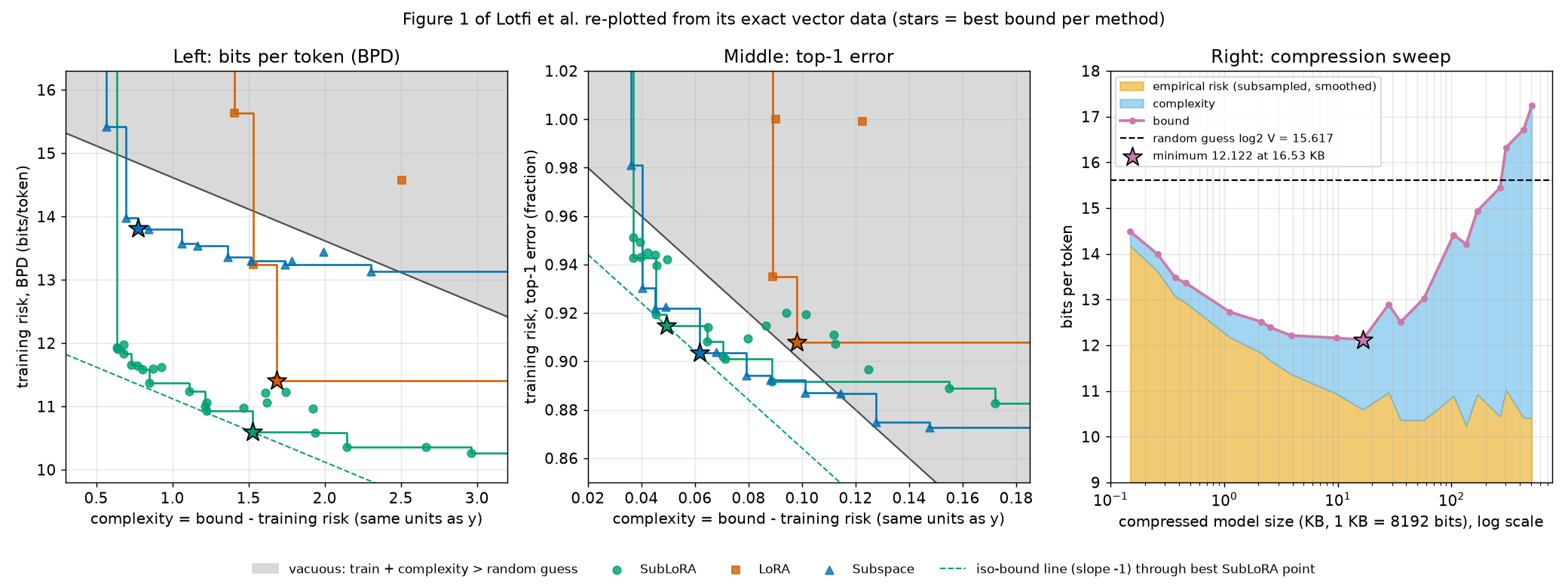
Our re-plot of Figure 1 from the exact plotted data (ch23_fig1.py). Same data as the paper's figure; colours, markers, frontier staircases, stars and the dashed iso-bound line are ours.

PAPER §1, p. 2, Figure 1 and caption The left two panels show, for many trained GPT-2-small models, the "complexity" (horizontal) against the training loss (vertical), for SubLoRA, LoRA alone and subspace training alone. The bound is the sum of the two coordinates, lower is better, and the shaded region marks where the bound is vacuous. The caption calls the cloud the Pareto frontier of complexity and empirical risk. The right panel shows, for SubLoRA, how the bound and its two parts change as the degree of compression is varied, and that an intermediate degree is optimal.

MY EXPLANATION How to read the left panels, step by step:

1. Each dot is one trained-and-compressed model (one run with particular hyperparameters such as \(d\), \(r\), learning rate, \(\alpha\)). All are GPT-2-small architectures; the colour says which compression scheme was used.
2. Vertical position = the model's training loss: the smoothed BPD or the top-1 error, averaged over the \(n=10{,}000\) subsampled training documents. This is \(\hat{\hat R}(h)\) of Chapter 17.
3. Horizontal position = everything the bound adds to that training loss, in the same units. For the BPD panel it is bits per token; for the top-1 panel it is a fraction.
4. The bound is \(x+y\). So every line of slope \(-1\) is a line of equal bound (an iso-bound line). Moving down-left along any direction improves the bound; moving along a slope \(-1\) line leaves it unchanged.
5. The shaded region is everything above the iso-bound line at the random-guess level: \(x + y > \log_2 V\) (BPD) or \(x+y > 1-1/V\) (top-1). A dot inside it has a vacuous bound.
6. The best model of a method is the dot that the lowest iso-bound line touches. That dot is always on the method's Pareto frontier (proof in the deeper block).

MY EXPLANATION A Pareto frontier is defined like this. Point \(q\) dominates point \(p\) if \(q\) is at least as good on both coordinates and strictly better on one (here: \(q\) has complexity \(\le\) and training loss \(\le\) those of \(p\), not both equal). The Pareto frontier of a set of points is the set of points that no other point dominates. Drawn as a staircase, it is the lower-left edge of the cloud. One method's frontier dominates another's if every point of the second is dominated by some point of the first.

MY EXPLANATION The right panel is different. Its horizontal axis is the model's compressed size in KB (log scale), not the complexity term. For each model the empirical risk (orange in our plot) and the complexity (blue) are stacked, so the top edge is the bound. Small models have low complexity but high training loss; large ones the reverse; the bound is lowest in between.

Paper erratum E60 (same issue as E57): the x-axis of Figure 1 (left) is not 'the 2nd term in Equation 1'

PAPER Figure 1 caption, p. 2 The caption calls the horizontal coordinate the 2nd term in Equation 1. MY EXPLANATION The plotted values equal the sum of both extra terms of the subsampling bound, Eq. (3): the prior term over \(m\) documents and the Hoeffding term over the \(n\) subsampled documents. For the best BPD model (16.5325 KB, \(\alpha = 0.25\), \(\Delta = 17.2020\)) the plotted value is 1.5278; Eq. (3)'s two terms give 1.3171 + 0.2106 = 1.5276 (the sum of the unrounded terms); Eq. (1)'s second term alone would be 1.3170 (output [5]). Chapter 20 found the same issue independently (erratum E57). The same holds in the top-1 panel (0.0494 plotted, 0.0371 + 0.0122 = 0.0493). The vertical axis "BPD (train)" is likewise the subsampled, smoothed empirical risk, not Eq. (1)'s full-data \(\hat R\). No number in the paper changes; the label understates what the horizontal axis contains.

Paper erratum E61: the shaded region of Figure 1 (left) is truncated

MY EXPLANATION In the top-1 panel the shading follows the line \(x+y = 1-1/V\) only up to complexity 0.1336; from there to 0.1790 it has a flat floor at 0.8664 (output [2]). In the BPD panel the shading stops at train 15.9036 and complexity 3.0815. So the picture shows less vacuous area than the rule defines: a model at complexity 0.17 with training error 0.85 would be vacuous (\(0.17+0.85 > 1\)) but would sit below the drawn shading. No plotted point is affected: for all 40 points in each panel, "inside the drawn shading" agrees with "sum above the random-guess level" (output [3]).

Paper errata E25 and E62: the right panel's sweep is not described, and it mixes d and α

PAPER Figure 1 caption, p. 2 The caption says the panel varies the extent of compression "for a fixed model" but does not say how the sweep was produced (E25). MY EXPLANATION The data tell us more. Eight of the 20 sweep points are exactly the eight \(d\) values of Figure 2 (left), same sizes and same bounds (output [6]). And inverting Eq. (3) for each point's interval width \(\Delta\) (deeper block below) gives values that match \(\alpha = 0.25\) (\(\Delta = 17.202\)) for 14 points and \(\alpha = 0.5\) (\(\Delta = 15.617\)) for 6 points, the smallest and the five largest (output [6]). So "fixed model" can only mean a fixed architecture: the points differ in \(d\) and in \(\alpha\), each presumably at its best \(\alpha\), as erratum E41 found for Figure 2 (right).

Worked example with real numbers

Everything in this section is MY EXPLANATION; every number is from ch23_fig1.py's output (shown at the end) unless another script is named. Units: BPD values in bits per token; top-1 values as fractions.

(a) Figure 1 reproduces Table 1

For each method, take the dot with the smallest \(x + y\) (output [1]):

Panel	Method	dots	train	+ complexity	= bound	Table 1
BPD	SubLoRA	24	10.5945	1.5278	12.1224	12.12
BPD	LoRA	4	11.4091	1.6856	13.0947	13.09
BPD	Subspace	12	13.8138	0.7758	14.5896	14.59
Top-1	SubLoRA	24	0.9148	0.0494	0.9641	96.41 %
Top-1	LoRA	4	0.9078	0.0980	1.0058	100 %
Top-1	Subspace	12	0.9037	0.0616	0.9652	96.52 %

Every entry rounds to Table 1 (the script asserts it). The one exception is instructive: LoRA's best top-1 bound is 1.0058, above 1. An error rate is never above 1, so Table 1 reports it as 100 % — vacuous in every sense. Note also the unequal effort: 24 SubLoRA runs, 12 subspace runs, 4 LoRA runs.

(b) The shaded boundary is the line "bound = random guess"

The lower edge of the extracted BPD shading is a straight line through 100 vertices with slope \(-1.00000\) and intercept 15.61703 (output [2]). \(\log_2 50{,}257 = 15.61704\). The top-1 edge has slope \(-1.00001\) and intercept 0.99998 \(= 1 - 1/50{,}257\). So the shading is exactly the set where train + complexity exceeds the random-guess level.

Counting dots above that level (output [3]): BPD — SubLoRA 0 of 24, LoRA 2 of 4, Subspace 1 of 12; top-1 — SubLoRA 8 of 24, LoRA 4 of 4, Subspace 4 of 12. This matches the text's claim that LoRA alone is vacuous for top-1.

(c) What the complexity coordinate contains

Take the best BPD model: compressed size 16.5325 KB (Figure 2), \(\alpha = 0.25\), so \(\Delta = 17.2020\) bits per token (Chapter 16). With \(\delta = 0.05\) and \(m = 8{,}009{,}762\) SOURCE: authors' code / nanoGPT, \(n = 10{,}000\) PAPER §6.1, natural logs and 1 KB = 8192 bits SOURCE: Lotfi et al. 2022; erratum E35 (output [5]):

• prior term over the \(m\) documents: 1.3171 bits per token;
• Hoeffding term over the \(n\) subsampled documents: 0.2106 bits per token;
• sum 1.5276 (adding the unrounded terms), against the plotted 1.5278.

Reading a bound off the figure: the dashed iso-bound line through SubLoRA's star meets the vertical axis (\(x=0\)) at 12.1224, the bound.

(d) Pareto frontiers: decisive for BPD, a tie for top-1

Output [4] lists each method's frontier and asks: is each LoRA or subspace dot dominated by some SubLoRA dot?

• BPD panel. All 4 LoRA dots and 11 of 12 subspace dots are dominated. The exception, (0.5652, 15.4148), is a subspace dot with smaller complexity than any SubLoRA dot — and it is vacuous anyway. SubLoRA also reaches the lowest training loss: 10.2622 versus 11.4091 (LoRA) and 13.1318 (subspace). This is what the contributions mean by subspace training alone giving a "high value of empirical BPD".
• Top-1 panel. All 4 LoRA dots are dominated, but only 1 of 12 subspace dots. The two frontiers cross: subspace training reaches lower training error at large complexity (0.8728 versus 0.8828). SubLoRA still has the lowest bound, 0.9641 versus 0.9652, a margin of 0.0011 (0.11 percentage points), from single runs. For BPD the margin is 2.4672 bits per token.

So the caption's headline (SubLoRA finds solutions with both low training error and low complexity) is strongly supported for BPD and only marginally for top-1 error.

(e) The compression sweep

The right panel has 20 models from 0.148 KB to 509.4 KB (output [6]). The bound falls from 14.4895 at the smallest model to its minimum 12.1223 at 16.53 KB (empirical 10.5945 + complexity 1.5278 — the same model as the best dot on the left), then rises to 17.2395 at the largest. Three models (301, 432 and 509 KB) are vacuous: their complexity has grown so large that the bound passes 15.617. In the re-plot, the orange band (training loss) barely moves to the right of the minimum while the blue band (complexity) keeps widening — the reason an intermediate size wins.

(f) Why classical counting is hopeless here

For contrast, the plain counting bound of Chapter 10 for GPT-2 small stored as float32 numbers gives a gap term of 13.0867 even for a loss in \([0,1]\) (output [6] of ch10_union.py): a bound on an error rate above 13. Compression, not counting, is what makes Figure 1's complexities as small as 1.5 bits per token.

Going deeper

This hub collects the derivations behind the definitions above. Everything here is MY EXPLANATION unless tagged.

Going deeper: VC dimension, shattering and the VC bound

Setting. Inputs \(z\) from a set \(\mathcal Z\); a class \(\mathcal H\) of classifiers \(h:\mathcal Z\to\{0,1\}\); the 0-1 loss.

Shattering. A finite set \(S = \{z_1,\dots,z_k\}\) is shattered by \(\mathcal H\) if for every labelling \((y_1,\dots,y_k)\in\{0,1\}^k\) some \(h\in\mathcal H\) has \(h(z_j)=y_j\) for all \(j\). There are \(2^k\) labellings, so shattering needs at least \(2^k\) distinct behaviours on \(S\).

VC dimension. \(d_{\mathrm{VC}}(\mathcal H)\) is the largest \(k\) such that some set of \(k\) inputs is shattered (infinite if there is no largest).

Example. Thresholds on the real line, \(h_t(z) = \mathbf 1[z\ge t]\). One point is shattered (put \(t\) below or above it). Two points \(z_1<z_2\) are not: the labelling \((1,0)\) needs \(z_1\ge t > z_2\), impossible. So \(d_{\mathrm{VC}} = 1\).

Growth function. \(\Pi_{\mathcal H}(k)\) = the largest number of distinct labellings \(\mathcal H\) produces on any \(k\) inputs. Shattering means \(\Pi_{\mathcal H}(k)=2^k\). The Sauer–Shelah lemma says that if \(d_{\mathrm{VC}} = d < \infty\) then

\[ \Pi_{\mathcal H}(k) \le \sum_{i=0}^{d}\binom{k}{i} \le \Big(\frac{ek}{d}\Big)^{d}\quad (k\ge d), \]

so the number of behaviours grows only polynomially in \(k\) once \(k\) passes \(d\). (Proof skipped: the first inequality is a standard induction on \(k\); the second follows from \(\sum_{i\le d}\binom{k}{i}(d/k)^d \le \sum_{i\le d}\binom{k}{i}(d/k)^i \le (1+d/k)^k \le e^d\).)

The VC bound (shape). With probability at least \(1-\delta\) over the random draw of \(m\) i.i.d. training examples, simultaneously for all \(h\in\mathcal H\),

\[ R(h) \le \hat R(h) + c\,\sqrt{\frac{d\,\ln(2em/d) + \ln(4/\delta)}{m}}, \]

where \(c\) is a universal constant whose value differs between textbooks. Proof sketch, with what is skipped: (1) symmetrization — the probability that some \(h\) has a large gap between its true and training risk is at most twice the probability that it has a large gap between its errors on the training sample and on an independent "ghost" sample of the same size (skipped: the conditioning argument behind the factor 2); (2) on the \(2m\) points of both samples, \(\mathcal H\) behaves as at most \(\Pi_{\mathcal H}(2m)\) distinct classifiers, so a union bound (Chapter 10) over those behaviours costs \(\ln \Pi_{\mathcal H}(2m)\le d\ln(2em/d)\) nats; (3) for each behaviour, randomly swapping examples between the two samples gives a Hoeffding-type tail (Chapter 9).

Compare with Eq. (1): there the price of a hypothesis is \(\ln(1/P(h))\), different for each \(h\); here every \(h\) pays the same \(d\ln(2em/d)\), determined by the whole class.

Why it is vacuous for networks. Zhang et al. (2021) showed that standard networks can reach zero training error on random labels, so they shatter their training inputs: \(d_{\mathrm{VC}}\ge m\). Then \(d\ln(2em/d)/m = \ln(2e) = 1+\ln 2 > 1\) at \(d = m\), and the bound exceeds 1 for any \(c\ge1\). More fundamentally, Chapter 2's deeper block proves that no bound that depends only on the class, \(m\) and \(\delta\) can beat \(\tfrac12\) for a class that shatters. SOURCE: Bartlett, Harvey, Liaw & Mehrabian 2019 For piecewise-linear networks the VC dimension grows at least proportionally to the number of parameters times the depth (up to a log factor), which for GPT-2 small is far above the \(m = 8{,}009{,}762\) documents.

Going deeper: Rademacher complexity, and why fitting random labels makes it maximal

Rademacher variables. \(\varepsilon_1,\dots,\varepsilon_m\) independent, each \(+1\) or \(-1\) with probability \(\tfrac12\) (fair coins).

Definition. For a class \(\mathcal F\) of functions \(f:\mathcal Z\to\mathbb R\) and a fixed sample \(S = (z_1,\dots,z_m)\), the empirical Rademacher complexity is

\[ \hat{\mathfrak R}_S(\mathcal F) = \mathbb E_{\varepsilon}\Big[\sup_{f\in\mathcal F}\frac1m\sum_{j=1}^m \varepsilon_j f(z_j)\Big]. \]

The expectation is over the coins only; \(S\) is fixed. In words: draw random signs, let the class pick its member most correlated with them, and average that best correlation. The Rademacher complexity \(\mathfrak R_m(\mathcal F)\) is the average of \(\hat{\mathfrak R}_S\) over random samples \(S\) of size \(m\).

The bound (Bartlett & Mendelson, 2002). If every \(f\in\mathcal F\) takes values in \([0,1]\), then with probability at least \(1-\delta\) over the random draw of \(S\), simultaneously for all \(f\in\mathcal F\),

\[ \mathbb E[f(z)] \le \frac1m\sum_{j=1}^m f(z_j) + 2\,\mathfrak R_m(\mathcal F) + \sqrt{\frac{\ln(1/\delta)}{2m}}. \]

Proof sketch, with what is skipped: the worst gap \(G(S)=\sup_f(\mathbb E f - \frac1m\sum_j f(z_j))\) changes by at most \(1/m\) when one example is replaced, so McDiarmid's inequality (a generalization of Hoeffding's inequality proved by the same Chernoff method, Chapter 9; its proof is skipped here) gives \(G(S)\le\mathbb E[G]+\sqrt{\ln(1/\delta)/(2m)}\). Then a ghost sample and random sign swaps show \(\mathbb E[G]\le 2\mathfrak R_m(\mathcal F)\) (skipped: the symmetrization computation).

Fitting random labels makes it maximal. Write a classifier in sign form, \(g_h(z) = 2h(z)-1\in\{-1,+1\}\), and labels as \(y'_j = 2y_j - 1\in\{-1,+1\}\). Suppose \(\mathcal H\) shatters \(S\). For any sign pattern \(\varepsilon\) choose \(h\) with \(g_h(z_j)=\varepsilon_j\); then \(\frac1m\sum_j \varepsilon_j g_h(z_j) = \frac1m\sum_j 1 = 1\), the largest possible value. Hence \(\hat{\mathfrak R}_S(\{g_h\}) = 1\).

Now the 0-1 loss: \(\mathbf 1[h(z_j)\ne y_j] = \tfrac12(1 - y'_j g_h(z_j))\), because \(y'_j g_h(z_j)=+1\) when they agree and \(-1\) when they disagree. So

\[ \begin{aligned} \hat{\mathfrak R}_S(\text{loss class}) &= \mathbb E_\varepsilon\Big[\sup_h \frac1m\sum_j \varepsilon_j\tfrac12\big(1 - y'_j g_h(z_j)\big)\Big]\\ &= \mathbb E_\varepsilon\Big[\frac1{2m}\sum_j \varepsilon_j\Big] + \tfrac12\,\mathbb E_\varepsilon\Big[\sup_h \frac1m\sum_j (-\varepsilon_j y'_j)\, g_h(z_j)\Big]\\ &= 0 + \tfrac12\cdot 1 = \tfrac12 . \end{aligned} \]

Line 2 splits the sum; the first part does not depend on \(h\) and has expectation 0. Line 3 uses that \(-\varepsilon_j y'_j\) is again a fair \(\pm1\) coin sequence (multiplying a fair coin by a fixed sign leaves it fair), so the second expectation is \(\hat{\mathfrak R}_S(\{g_h\}) = 1\). The bound's middle term is then \(2\cdot\tfrac12 = 1\): the bound on an error rate is at least 1, i.e. vacuous.

Going deeper: sub-Gaussian variables, and why the NLL is not known to be one

Definition. A random variable \(X\) with mean \(\mu\) is sub-Gaussian with variance proxy \(\sigma^2\) if its moment generating function (Chapter 9) satisfies

\[ \mathbb E\big[e^{\lambda (X-\mu)}\big] \le e^{\lambda^2\sigma^2/2}\quad\text{for every real }\lambda . \]

A normal variable with variance \(\sigma^2\) meets this with equality.

Tail bound. For \(t>0\) and any \(\lambda>0\), Markov's inequality applied to \(e^{\lambda(X-\mu)}\) gives \(\Pr[X-\mu\ge t]\le e^{-\lambda t}\,\mathbb E[e^{\lambda(X-\mu)}]\le e^{-\lambda t + \lambda^2\sigma^2/2}\). The exponent is smallest at \(\lambda = t/\sigma^2\), where it equals \(-t^2/(2\sigma^2)\). So \(\Pr[X-\mu\ge t]\le e^{-t^2/(2\sigma^2)}\).

Averages. If \(X_1,\dots,X_m\) are independent, each sub-Gaussian with proxy \(\sigma^2\), the average \(\bar X\) satisfies \(\mathbb E[e^{\lambda(\bar X-\mu)}] = \prod_j \mathbb E[e^{(\lambda/m)(X_j-\mu)}]\le e^{m(\lambda/m)^2\sigma^2/2} = e^{\lambda^2(\sigma^2/m)/2}\), so it is sub-Gaussian with proxy \(\sigma^2/m\) and \(\Pr[\bar X-\mu\ge t]\le e^{-mt^2/(2\sigma^2)}\).

Bounded variables. Hoeffding's lemma (proved in Chapter 9) says that \(X\in[a,b]\) has \(\mathbb E[e^{\lambda(X-\mu)}]\le e^{\lambda^2(b-a)^2/8}\), i.e. it is sub-Gaussian with \(\sigma = (b-a)/2\). Plugging \(\sigma = \Delta/2\) into the average bound gives \(e^{-2mt^2/\Delta^2}\) — Hoeffding's inequality. So the paper's route (force boundedness by smoothing) is the special case of the sub-Gaussian route in which the proxy is known for every model.

Why the NLL is a problem. For a fixed model with finitely many inputs, the NLL is bounded, hence sub-Gaussian — but with \(\sigma\) equal to half the worst-case loss, which can be astronomically large (Chapter 6: one token with probability below \(10^{-440.3}\) is enough to push a 100-token document past 15.617 bits per token; and in float32 a probability can round to exactly 0, giving infinite loss). A useful, small \(\sigma\) would have to come from the data distribution making such documents rare, which is an unverifiable assumption about text. That is the sense of the paper's "no clear analogous tail behavior".

Going deeper: Haddouche et al.'s range Q(h) and why it explodes with depth

The idea. PAPER §2, p. 3 If \(\sup_x R(h,x)\le Q(h)\) for every input \(x\), a PAC-Bayes bound can be built with \(Q(h)\) in the role of the range, even when \(\sup_h Q(h) = \infty\). MY EXPLANATION For one fixed \(h\) this is Hoeffding with \(\Delta = Q(h)\); the work of Haddouche et al. is to make it hold for a data-dependent choice of \(h\). Either way the deviation term is proportional to \(Q(h)\).

From logits to worst-case loss. With logits \(z_1,\dots,z_V\), the softmax probability of token \(i\) is

\[ p_i = \frac{e^{z_i}}{\sum_{j=1}^V e^{z_j}} \ge \frac{e^{z_i}}{V e^{z_{\max}}} = \frac{e^{-(z_{\max}-z_i)}}{V}, \]

because each of the \(V\) terms in the denominator is at most \(e^{z_{\max}}\). Taking \(-\log_2\): \(-\log_2 p_i \le \log_2 V + (z_{\max}-z_{\min})/\ln 2\) bits. So the worst-case loss is controlled by the spread of the logits.

Lipschitz constants multiply. A function \(f\) is \(K\)-Lipschitz if \(\lVert f(u)-f(v)\rVert\le K\lVert u-v\rVert\) for all \(u, v\). If \(f\) is \(K_f\)-Lipschitz and \(g\) is \(K_g\)-Lipschitz, then \(\lVert f(g(u))-f(g(v))\rVert\le K_f\lVert g(u)-g(v)\rVert\le K_fK_g\lVert u-v\rVert\). By induction, a stack of \(L\) layers with constants \(K_1,\dots,K_L\) is \(K_1\cdots K_L\)-Lipschitz. The resulting bound on the logit spread, and hence on \(Q(h)\), can grow like a product over layers — exponentially in depth. With a factor of 2 per layer the product is 4,096 at 12 layers, 16,777,216 at 24, 68,719,476,736 at 36 and 281,474,976,710,656 at 48 (output [0]). These are illustrations of the growth, not measured constants of GPT-2.

Consequence. The bound's complexity term is \(\Delta\sqrt{\cdots}\). With \(\Delta\) replaced by a \(Q(h)\) of thousands of bits per token or more, the term alone exceeds the random-guess level of 15.617. Prediction smoothing instead gives every hypothesis the same small width, \(\Delta(0.25) = 17.202\) (output [0]).

Going deeper: Pareto frontiers and why the best bound sits on one

Setting. A finite set of points \(p = (x_p, y_p)\) (complexity, training loss); the bound of point \(p\) is \(b(p) = x_p + y_p\).

Claim 1: a minimizer of \(b\) lies on the Pareto frontier. Let \(p^{\star}\) minimize \(b\) (a finite set has a minimizer). If \(p^{\star}\) were dominated by some \(q\), then \(x_q\le x_{p^{\star}}\) and \(y_q\le y_{p^{\star}}\) with at least one inequality strict, so \(b(q) = x_q + y_q < x_{p^{\star}} + y_{p^{\star}} = b(p^{\star})\). That contradicts the minimality of \(p^{\star}\). So every minimizer is undominated, i.e. on the frontier.

Claim 2: it lies on the lower-left convex hull. The set \(\{(x,y): x+y = b(p^{\star})\}\) is a line of slope \(-1\) with every point of the set on or above it. So \(p^{\star}\) is a point where a supporting line of slope \(-1\) touches the cloud. Frontier points in a "dent" of the staircase (strictly above the segment joining two neighbours) can never be optimal for any weighted sum \(w_1x + w_2y\) with positive weights.

Claim 3: frontier dominance implies a better best bound, not conversely. If every point of method B is dominated by a point of method A, then \(\min_A b\le\min_B b\) (apply Claim 1's inequality to B's minimizer). The converse fails: in the top-1 panel SubLoRA has the lower minimum (0.9641 versus 0.9652) although its frontier does not dominate subspace training's (output [4]).

Caveats for reading Figure 1. The frontier is that of the runs that were tried, not of the method. More runs can only push a frontier down-left, and the methods got very different numbers of runs (24, 12 and 4, output [1]). Each point is a single run; no seeds or error bars are shown.

Going deeper: recovering Δ and α from the right panel

For a point of the right panel we can read the compressed size (KB) on the horizontal axis and the empirical risk \(\hat{\hat R}\) and bound \(B\) on the vertical one. Eq. (3) of Chapter 17 says

\[ B - \hat{\hat R} = \Delta\cdot g(C),\qquad g(C) = \sqrt{\frac{C\ln 2 + 2\ln C + \ln\frac{1}{s\delta}}{2m}} + \sqrt{\frac{\ln\frac{1}{(1-s)\delta}}{2n}}, \]

with \(C\) = size in bits (KB × 8192), \(s = n/(n+m)\), and \(\ln\) the natural log (the bound's log must be \(\ln\) because it comes from Hoeffding's \(e^{-2mt^2/\Delta^2}\); erratum E02). Here the probability is over the random draw of the \(m\) documents and of the subsample; the model is fixed. Everything except \(\Delta\) is known, so \(\hat\Delta = (B-\hat{\hat R})/g(C)\), in bits per token. Then compare with the grid \(\Delta(\alpha) = \log_2(1+(1-\alpha)V/\alpha)\) for \(\alpha\in\{10^{-4},\dots,0.5\}\).

Result (output [6]): 14 points give \(\hat\Delta\) within \(+0.00\) % to \(+0.50\) % of \(\Delta(0.25)=17.202\), and 6 points within \(+0.00\) % to \(+0.75\) % of \(\Delta(0.5) = 15.617\); no other grid value is close. The small positive deviations are largest for the smallest models. [MY EXPLANATION, unverified conjecture] That pattern fits a prior that charges a few dozen bits more than \(C + 2\log_2 C\) (for example for hyperparameter choices, Chapter 24): a fixed number of extra bits matters relatively more when \(C\) is small.

Common misconceptions

• Misconception: Each dot in Figure 1 (left) is a different architecture. — Actually: every dot is a GPT-2-small architecture trained and compressed with one setting of the hyperparameters; dots differ in the compression scheme (colour), subspace dimension, rank, learning rate, \(\alpha\) and so on.
• Misconception: The "Complexity" axis is the model's size. — Actually: it is the bound's penalty, in the same units as the loss (bits per token or error fraction). It grows like the square root of the compressed size and also contains the subsampling term (worked example (c)); the model size is the right panel's axis.
• Misconception: A dot in the shaded region is a model that does not generalize. — Actually: the shading says only that this certificate is uninformative. The model may generalize well; the bound just cannot show it.
• Misconception: A non-vacuous bound "for an 849M-parameter model" certifies an 849M-parameter LLM as it is normally used. — Actually: it certifies the SubLoRA-compressed, quantized, smoothed model that the few-KB message rebuilds; its loss is far worse than a normally trained model's (Chapter 25).
• Misconception: The paper needs PAC-Bayes. — Actually: it borrows the prior idea from PAC-Bayes but uses a finite-hypothesis bound, Eq. (1), for a single deterministic model (Chapter 11).
• Misconception: Compression for bounds is the same as compression for deployment. — Actually: deployment methods (QLoRA, GPTQ, SpQR, …) optimize speed and memory; a bound cares only about the number of bits in the description, even if decoding is slow.

Self-test

Q1. In the top-1 panel, LoRA's best dot has training error 0.9078 and complexity 0.0980. Is its bound vacuous? What does Table 1 report, and why?

Answer

The bound is \(0.9078 + 0.0980 = 1.0058\) (output [1]). The random-guess level is \(1-1/V = 0.99998\), so the bound is vacuous; it even exceeds 1, the largest possible error rate. Table 1 reports it as 100 %, since a bound above 100 % says nothing more than 100 %.

Q2. Why do VC-dimension and Rademacher bounds say nothing about networks that can fit random labels, while the paper's bound can still be non-vacuous for the same networks?

Answer

VC and Rademacher bounds charge every hypothesis the same price, computed from the whole class. If the class can fit any labelling of the training inputs, the VC dimension is at least \(m\) and the Rademacher complexity of the 0-1 loss class is \(\tfrac12\), so the bound's complexity term reaches 1 (deeper blocks). Eq. (1) instead charges each hypothesis \(\ln(1/P(h))\) with a prior that favours short descriptions. A network class that can fit random labels still contains hypotheses with short descriptions; if training finds one that also fits the real data, its price is small. The bound depends on which hypothesis was found, not only on what the class could fit.

Q3. In the top-1 panel, 11 of the 12 subspace dots are not dominated by any SubLoRA dot. Does this contradict the paper's claim that SubLoRA gives the best top-1 bound?

Answer

No. The best bound is the minimum of complexity + training error, which is attained on each method's frontier at the point touched by the lowest slope \(-1\) line. Frontier dominance would guarantee a better minimum, but a better minimum does not require dominance. Here the frontiers cross: subspace training reaches lower training error at high complexity, while SubLoRA's frontier comes slightly closer to the origin along the diagonal. Its best bound is 0.9641 against 0.9652 (output [1]), a margin of 0.11 percentage points from single runs — real in the reported data, but too small to call SubLoRA decisively better for top-1 error.

Code for this chapter

Run it from the project root:

.venv/Scripts/python explainer/code/ch23_fig1.py

It reads explainer/code/outputs/fig_extract.json (the exact plotted coordinates, produced by fig_extract.py), asserts agreement with Table 1 and with the random-guess lines, and writes the re-plotted figure.

Source: ch23_fig1.py

"""Chapter 23 demo: reading Figure 1 of arXiv 2312.17173 from its exact plotted data.

Claims reproduced / checked (all from the vector data extracted by fig_extract.py, which this script only reads):
  [1] The best point (minimum train + complexity) of each method in Figure 1 (left) rounds to Table 1:
      BPD 12.12 / 13.09 / 14.59 and Top-1 96.41 / 100 (sum >= 1) / 96.52 (%).
  [2] The shaded "vacuous" region is bounded by a line of slope -1 through (0, log2 V) (BPD panel) and
      (0, 1 - 1/V) (Top-1 panel), i.e. it is exactly {train + complexity >= random-guess level}.
  [3] Which points are vacuous, per method.
  [4] The Pareto frontier of each method and whether SubLoRA's frontier dominates the others.
  [5] The plotted "Complexity" equals BOTH extra terms of Eq. (3), not only the second term of Eq. (1)
      (caption wording; new erratum logged by Ch. 23).
  [6] Figure 1 (right): the compression sweep, its minimum (12.122 at 16.53 KB), the implied interval width
      Delta and smoothing weight alpha of each point, and the overlap with Figure 2 (left).
Writes outputs/ch23_fig1.txt and docs/assets/fig/ch23_fig1_replot.png.
"""
from __future__ import annotations

import json
import math
import subprocess
import sys
from pathlib import Path

HERE = Path(__file__).resolve().parent
sys.path.insert(0, str(HERE))
import pacbound as pb  # noqa: E402

import numpy as np  # noqa: E402
import matplotlib  # noqa: E402

matplotlib.use("Agg")
import matplotlib.pyplot as plt  # noqa: E402

JSON = HERE / "outputs" / "fig_extract.json"
OUT_TXT = HERE / "outputs" / "ch23_fig1.txt"
FIG = HERE.parent / "docs" / "assets" / "fig" / "ch23_fig1_replot.png"

if not JSON.exists():  # produced by the orchestrator's extractor; run it if missing
    subprocess.run([sys.executable, str(HERE / "fig_extract.py")], check=True)
data = json.loads(JSON.read_text(encoding="utf-8"))
F1 = data["figure1"]

lines: list[str] = []


def out(s: str = "") -> None:
    print(s)
    lines.append(s)


V = pb.V_GPT2
RG_BPD = pb.random_guess_bpd(V)              # bits/token
RG_TOP1 = pb.random_guess_topk_error(1, V)  # fraction
METHODS = ["SubLoRA", "LoRA", "Subspace"]
KB_BITS = 8192                               # [SOURCE: Lotfi et al. 2022; erratum E35] bits per KB

# --------------------------------------------------------------------------------------------
# [0] context numbers used in the walkthrough of the Abstract and Sections 1-2
# --------------------------------------------------------------------------------------------
D_SMALL = pb.gpt2_params(12, 768)
out("[0] Context: V = 50,257 [SOURCE: GPT-2 tokenizer]; random guess: log2 V = "
    f"{RG_BPD:.4f} bits/token, top-1 error 1 - 1/V = {RG_TOP1:.6f}")
out(f"    OpenWebText train tokens {pb.OWT_TRAIN_TOKENS:,} [SOURCE: nanoGPT]; documents m = {pb.M_DOCS:,} [SOURCE]; "
    f"tokens/doc {pb.OWT_TRAIN_TOKENS / pb.M_DOCS:.0f}")
out(f"    GPT-2 small parameters D = {D_SMALL:,} (nanoGPT count) = {D_SMALL / pb.M_DOCS:.1f} per training document")
lo, hi, wd = pb.smoothing_interval(0.25)
out(f"    smoothing, alpha = 0.25: per-token loss in ({lo:.3f}, {hi:.3f}) bits, width Delta = {wd:.3f} "
    "(same for every h)")
out("    Lipschitz products (illustration): per-layer factor 2 -> "
    + ", ".join(f"{L} layers: {2 ** L:,}" for L in (12, 24, 36, 48)))

# --------------------------------------------------------------------------------------------
# [1] best point per method vs Table 1
# --------------------------------------------------------------------------------------------
TABLE1 = {"bpd": {"SubLoRA": 12.12, "LoRA": 13.09, "Subspace": 14.59},          # [PAPER Table 1] bits/token
          "top1": {"SubLoRA": 96.41, "LoRA": 100.0, "Subspace": 96.52}}       # [PAPER Table 1] percent
out("[1] Best point per method in Fig. 1 (left) = min over points of (train + complexity)")
best = {}
for panel, key, unit, scale in [("bpd", "left_bpd", "bits/token", 1.0), ("top1", "left_top1", "fraction", 100.0)]:
    for meth in METHODS:
        pts = F1[key]["points"][meth]
        b = min(pts, key=lambda p: p["complexity"] + p["train_risk"])
        s = b["complexity"] + b["train_risk"]
        best[(panel, meth)] = b
        tab = TABLE1[panel][meth]
        if panel == "top1" and meth == "LoRA":
            assert s >= 1.0, "LoRA top-1 sum should exceed 1 (reported as 100 %)"
            note = "sum >= 1 -> reported as 100 (vacuous)"
        else:
            assert abs(round(s * scale, 2) - tab) < 1e-9, (panel, meth, s, tab)
            note = f"diff {s * scale - tab:+.4f}" + (" pct pts" if panel == "top1" else "")
        out(f"    {panel:4s} {meth:8s} n={len(pts):2d}  train {b['train_risk']:.4f} + complexity "
            f"{b['complexity']:.4f} = {s:.4f} {unit}  | Table 1: {tab}  ({note})")

# --------------------------------------------------------------------------------------------
# [2] vacuous-region boundary
# --------------------------------------------------------------------------------------------
out("[2] Shaded region: the extracted polygon and its sloped lower edge")


poly_info = {}
for panel, key, rg, name in [("bpd", "left_bpd", RG_BPD, "log2 V"), ("top1", "left_top1", RG_TOP1, "1 - 1/V")]:
    polys = F1[key]["vacuous_polygon"]
    assert len(polys) == 1
    a = np.unique(np.round(np.asarray(polys[0]), 9), axis=0)
    xmin, xmax, ymax = a[:, 0].min(), a[:, 0].max(), a[:, 1].max()
    lower = a[(a[:, 1] < ymax - 1e-6)]                       # vertices of the lower boundary
    ymin = lower[:, 1].min()
    floor = lower[np.abs(lower[:, 1] - ymin) < 1e-6]          # flat bottom, if any
    has_floor = len(floor) > 1 and np.ptp(floor[:, 0]) > 1e-3
    diag = lower[~(np.abs(lower[:, 1] - ymin) < 1e-6)] if has_floor else lower
    diag = diag[(diag[:, 0] > xmin + 1e-9) | (diag[:, 1] < ymax - 1e-6)]
    diag = diag[np.argsort(diag[:, 0])]
    diag = diag[~((np.abs(diag[:, 0] - xmax) < 1e-9) & (diag[:, 1] > diag[:, 1].min() + 1e-6))]
    slope, icpt = np.polyfit(diag[:, 0], diag[:, 1], 1)
    resid = np.max(np.abs(diag[:, 1] - (slope * diag[:, 0] + icpt)))
    poly_info[panel] = (xmin, xmax, ymax, floor[:, 0].min() if has_floor else None, ymin)
    out(f"    {panel:4s} shaded box: complexity {xmin:.4f}..{xmax:.4f}, top at train = {ymax:.4f}")
    out(f"         sloped edge: {len(diag)} vertices, slope {slope:.5f}, intercept {icpt:.5f}, max residual "
        f"{resid:.1e}; {name} = {rg:.5f} (diff {icpt - rg:+.5f})")
    assert abs(slope + 1) < 1e-3 and abs(icpt - rg) < 2e-4
_, xmax_t, _, xfloor, yfloor = poly_info["top1"]
out(f"    note: top-1 shading follows the line only up to complexity {xfloor:.4f}; from there to {xmax_t:.4f} it has "
    f"a flat floor at train = {yfloor:.4f}")

# --------------------------------------------------------------------------------------------
# [3] vacuous points per method
# --------------------------------------------------------------------------------------------
out("[3] Points whose train + complexity exceeds the random-guess level (vacuous) / total")
for panel, key, rg in [("bpd", "left_bpd", RG_BPD), ("top1", "left_top1", RG_TOP1)]:
    parts = []
    for meth in METHODS:
        pts = F1[key]["points"][meth]
        nv = sum(p["complexity"] + p["train_risk"] > rg for p in pts)
        parts.append(f"{meth} {nv}/{len(pts)}")
    out(f"    {panel:4s} (level {rg:.5f}): " + ", ".join(parts))
    # does the drawn shading agree with the arithmetic for every plotted point?
    from matplotlib.path import Path as MPath
    shade = MPath(np.asarray(F1[key]["vacuous_polygon"][0]))
    allp = [p for meth in METHODS for p in F1[key]["points"][meth]]
    agree = sum(bool(shade.contains_point((p["complexity"], p["train_risk"])))
                == (p["complexity"] + p["train_risk"] > rg) for p in allp)
    out(f"         drawn shading agrees with 'sum > level' for {agree}/{len(allp)} plotted points")
    assert agree == len(allp)

# --------------------------------------------------------------------------------------------
# [4] Pareto frontiers
# --------------------------------------------------------------------------------------------


def frontier(pts):
    """Non-dominated points (lower complexity AND lower train is better), sorted by complexity."""
    xy = sorted((p["complexity"], p["train_risk"]) for p in pts)
    fr, best_y = [], math.inf
    for x, y in xy:
        if y < best_y:
            fr.append((x, y))
            best_y = y
    return fr


def dominated_by(p, others):
    return any(q[0] <= p[0] and q[1] <= p[1] and (q[0] < p[0] or q[1] < p[1]) for q in others)


out("[4] Pareto frontiers (number of non-dominated points) and dominance by SubLoRA's points")
fronts = {}
for panel, key in [("bpd", "left_bpd"), ("top1", "left_top1")]:
    sub = [(p["complexity"], p["train_risk"]) for p in F1[key]["points"]["SubLoRA"]]
    msg = []
    for meth in METHODS:
        fronts[(panel, meth)] = frontier(F1[key]["points"][meth])
        msg.append(f"{meth} {len(fronts[(panel, meth)])} (lowest train {fronts[(panel, meth)][-1][1]:.4f})")
    out(f"    {panel:4s} frontier sizes: " + ", ".join(msg))
    for meth in ["LoRA", "Subspace"]:
        pts = [(p["complexity"], p["train_risk"]) for p in F1[key]["points"][meth]]
        undominated = [p for p in pts if not dominated_by(p, sub)]
        out(f"         {meth:8s} points dominated by some SubLoRA point: {len(pts) - len(undominated)}/{len(pts)}"
            + ("" if not undominated else "; not dominated: "
               + ", ".join(f"({x:.4f}, {y:.4f})" for x, y in undominated)))
    bs = {m: best[(panel, m)]["complexity"] + best[(panel, m)]["train_risk"] for m in METHODS}
    out(f"         best-bound margin Subspace - SubLoRA = {bs['Subspace'] - bs['SubLoRA']:.4f} "
        f"({'bits/token' if panel == 'bpd' else 'fraction'})")

# --------------------------------------------------------------------------------------------
# [5] What "Complexity" is
# --------------------------------------------------------------------------------------------
out("[5] Plotted 'Complexity' vs the terms of Eq. (1) and Eq. (3) (delta=0.05, m=8,009,762 [SOURCE: authors'")
out("    code / nanoGPT]; n=10,000; 1 KB = 8192 bits [SOURCE: Lotfi et al. 2022])")
for label, kb, width, plotted in [("BPD, d=50,000 model, 16.5325 KB, alpha=0.25", 16.5325,pb.smoothing_interval(0.25)[2],
                                   best[("bpd", "SubLoRA")]["complexity"]),
                                  ("Top-1 best SubLoRA point, taken to be the 3.878 KB (d=10,000) model, Delta=1", 3.878, 1.0,
                                   best[("top1", "SubLoRA")]["complexity"])]:
    lp = pb.log_inv_prior_nats_from_bits(kb * KB_BITS)
    t1, t2 = pb.eq3_terms(lp, pb.M_DOCS, pb.N_SUB, width=width)
    e1 = pb.eq1_complexity(lp, pb.M_DOCS, width=width)
    out(f"    {label}: Delta = {width:.4f}")
    out(f"       Eq.(3) term_m {t1:.4f} + term_n {t2:.4f} = {t1 + t2:.4f}; Eq.(1) 2nd term alone {e1:.4f}; "
        f"plotted {plotted:.4f} (diff vs Eq.3 {plotted - t1 - t2:+.4f})")
    assert abs(plotted - (t1 + t2)) < 2e-3 and abs(plotted - e1) > 0.01

# --------------------------------------------------------------------------------------------
# [6] Right panel: compression sweep
# --------------------------------------------------------------------------------------------
R = F1["right_sweep"]
bound = [(p["kb"], p["bpd"]) for p in R["bound"]]
area = R["empirical_risk_area"]
emp_by_kb = {round(p["kb"], 3): p["bpd"] for p in area if p["bpd"] > 10.0 + 1e-3}
sweep = [(kb, emp_by_kb[round(kb, 3)], b) for kb, b in bound]
rg_line = [h["bpd"] for h in R["horizontal_lines_bpd"] if h["colour"] == [0.1, 0.1, 0.1]][0]
kmin, emin, bmin = min(sweep, key=lambda t: t[2])
out(f"[6] Fig. 1 (right): {len(sweep)} models from {sweep[0][0]:.3f} to {sweep[-1][0]:.1f} KB; dashed line at "
    f"{rg_line:.4f} (log2 V = {RG_BPD:.4f})")
out(f"    bound {sweep[0][2]:.4f} at the smallest model, {sweep[-1][2]:.4f} at the largest; minimum bound {bmin:.4f} "
    f"bits/token at {kmin:.2f} KB")
out(f"    (empirical {emin:.4f} + complexity {bmin - emin:.4f})")
assert abs(rg_line - RG_BPD) < 1e-3 and abs(bmin - 12.122) < 5e-4 and abs(kmin - 16.53) < 5e-3
vac = [kb for kb, e, b in sweep if b > RG_BPD]
out(f"    vacuous sweep points (bound > log2 V): {len(vac)} (sizes {', '.join(f'{k:.0f}' for k in vac)} KB)")
# implied Delta: complexity / (Eq. 3 terms with width 1)
alpha_D = {a: pb.smoothing_interval(a)[2] for a in pb.ALPHA_GRID}
groups = {}
for kb, e, b in sweep:
    g = sum(pb.eq3_terms(pb.log_inv_prior_nats_from_bits(kb * KB_BITS), pb.M_DOCS, pb.N_SUB, width=1.0))
    Dimp = (b - e) / g
    a_near = min(alpha_D, key=lambda a: abs(alpha_D[a] - Dimp))
    groups.setdefault(a_near, []).append((kb, Dimp, (Dimp - alpha_D[a_near]) / alpha_D[a_near]))
for a, lst in groups.items():
    rel = [r for _, _, r in lst]
    out(f"    implied Delta nearest Delta(alpha={a}) = {alpha_D[a]:.3f}: {len(lst)} points, relative deviation "
        f"{min(rel) * 100:+.2f} % to {max(rel) * 100:+.2f} %; sizes (KB): "
        + ", ".join(f"{k:.3g}" for k, _, _ in lst))
# overlap with Figure 2 (left) and with the SubLoRA points of the left panel
f2 = data["figure2"]["left"] if "left" in data["figure2"] else None
f2kb = [p for p in (f2 or {}).get("compressed_size_kb", [])]
f2b = [p for p in (f2 or {}).get("bound", [])]
if f2kb and f2b:
    def val(p):
        return p["value"] if isinstance(p, dict) and "value" in p else p
    pairs = [(val(k), val(b)) for k, b in zip(f2kb, f2b)]
    diffs = []
    for k2, b2 in pairs:
        kb, e, b = min(sweep, key=lambda t: abs(math.log(t[0] / k2)))
        diffs.append((abs(kb - k2), abs(b - b2)))
    out(f"    Fig. 2 (left) models found in the sweep: {len(pairs)}/{len(pairs)}; max |size diff| "
        f"{max(d[0] for d in diffs):.3f} KB, max |bound diff| {max(d[1] for d in diffs):.4f} bits/token")
sub_bpd = [(p["complexity"], p["train_risk"]) for p in F1["left_bpd"]["points"]["SubLoRA"]]
shared = sum(any(abs((b - e) - x) < 2e-3 and abs(e - y) < 2e-3 for x, y in sub_bpd) for kb, e, b in sweep)
out(f"    sweep models that also appear as SubLoRA points in the left BPD panel: {shared}/{len(sweep)}")

OUT_TXT.write_text("\n".join(lines) + "\n", encoding="utf-8")

# --------------------------------------------------------------------------------------------
# Figure
# --------------------------------------------------------------------------------------------
COL = {"SubLoRA": "#009E73", "LoRA": "#D55E00", "Subspace": "#0072B2"}
MARK = {"SubLoRA": "o", "LoRA": "s", "Subspace": "^"}
plt.rcParams.update({"font.size": 11})
fig, axes = plt.subplots(1, 3, figsize=(16, 6.0))
for ax, panel, key, rg, ylab, xlim, ylim in [
        (axes[0], "bpd", "left_bpd", RG_BPD, "training risk, BPD (bits/token)", (0.3, 3.2), (9.8, 16.3)),
        (axes[1], "top1", "left_top1", RG_TOP1, "training risk, top-1 error (fraction)", (0.02, 0.185), (0.85, 1.02))]:
    xs = np.linspace(xlim[0], xlim[1], 200)
    ax.fill_between(xs, rg - xs, ylim[1], color="0.85", zorder=0, label="vacuous: train + complexity > random guess")
    ax.plot(xs, rg - xs, color="0.3", lw=1.2, zorder=1)
    for meth in METHODS:
        pts = F1[key]["points"][meth]
        ax.scatter([p["complexity"] for p in pts], [p["train_risk"] for p in pts], s=34, marker=MARK[meth],
                   color=COL[meth], alpha=0.8, zorder=3, label=meth)
        fr = fronts[(panel, meth)]
        fx = [fr[0][0]] + [p[0] for p in fr] + [xlim[1]]
        fy = [ylim[1]] + [p[1] for p in fr] + [fr[-1][1]]
        ax.step(fx, fy, where="post", color=COL[meth], lw=1.4, zorder=2)
        b = best[(panel, meth)]
        ax.scatter([b["complexity"]], [b["train_risk"]], s=210, marker="*", color=COL[meth], edgecolor="black",
                   zorder=4)
    b = best[(panel, "SubLoRA")]
    sbest = b["complexity"] + b["train_risk"]
    ax.plot(xs, sbest - xs, ls="--", color=COL["SubLoRA"], lw=1.1, zorder=1,
            label="iso-bound line (slope -1) through best SubLoRA point")
    ax.set_xlim(*xlim)
    ax.set_ylim(*ylim)
    ax.set_xlabel("complexity = bound - training risk (same units as y)")
    ax.set_ylabel(ylab)
    ax.grid(alpha=0.3)
axes[0].set_title("Left: bits per token (BPD)")
axes[1].set_title("Middle: top-1 error")
handles, labels = axes[1].get_legend_handles_labels()
fig.legend(handles, labels, loc="lower center", ncol=5, fontsize=9.5, frameon=False)
ax = axes[2]
kb = np.array([t[0] for t in sweep])
em = np.array([t[1] for t in sweep])
bd = np.array([t[2] for t in sweep])
ax.fill_between(kb, 9.0, em, color="#E69F00", alpha=0.55, label="empirical risk (subsampled, smoothed)")
ax.fill_between(kb, em, bd, color="#56B4E9", alpha=0.55, label="complexity")
ax.plot(kb, bd, color="#CC79A7", lw=2, marker="o", ms=4, label="bound")
ax.axhline(RG_BPD, ls="--", color="black", lw=1.2, label=f"random guess log2 V = {RG_BPD:.3f}")
ax.scatter([kmin], [bmin], s=210, marker="*", color="#CC79A7", edgecolor="black", zorder=5,
           label=f"minimum {bmin:.3f} at {kmin:.2f} KB")
ax.set_xscale("log")
ax.set_ylim(9.0, 18.0)
ax.set_xlabel("compressed model size (KB, 1 KB = 8192 bits), log scale")
ax.set_ylabel("bits per token")
ax.set_title("Right: compression sweep")
ax.legend(fontsize=8.5, loc="upper left")
ax.grid(alpha=0.3, which="both")
fig.suptitle("Figure 1 of Lotfi et al. re-plotted from its exact vector data (stars = best bound per method)",
             fontsize=12)
fig.tight_layout(rect=(0, 0.07, 1, 1))
FIG.parent.mkdir(parents=True, exist_ok=True)
fig.savefig(FIG, dpi=130)
print(f"figure written to {FIG}")

Output:

[0] Context: V = 50,257 [SOURCE: GPT-2 tokenizer]; random guess: log2 V = 15.6170 bits/token, top-1 error 1 - 1/V = 0.999980
    OpenWebText train tokens 9,035,582,198 [SOURCE: nanoGPT]; documents m = 8,009,762 [SOURCE]; tokens/doc 1128
    GPT-2 small parameters D = 123,689,472 (nanoGPT count) = 15.4 per training document
    smoothing, alpha = 0.25: per-token loss in (0.415, 17.617) bits, width Delta = 17.202 (same for every h)
    Lipschitz products (illustration): per-layer factor 2 -> 12 layers: 4,096, 24 layers: 16,777,216, 36 layers: 68,719,476,736, 48 layers: 281,474,976,710,656
[1] Best point per method in Fig. 1 (left) = min over points of (train + complexity)
    bpd  SubLoRA  n=24  train 10.5945 + complexity 1.5278 = 12.1224 bits/token  | Table 1: 12.12  (diff +0.0024)
    bpd  LoRA     n= 4  train 11.4091 + complexity 1.6856 = 13.0947 bits/token  | Table 1: 13.09  (diff +0.0047)
    bpd  Subspace n=12  train 13.8138 + complexity 0.7758 = 14.5896 bits/token  | Table 1: 14.59  (diff -0.0004)
    top1 SubLoRA  n=24  train 0.9148 + complexity 0.0494 = 0.9641 fraction  | Table 1: 96.41  (diff +0.0032 pct pts)
    top1 LoRA     n= 4  train 0.9078 + complexity 0.0980 = 1.0058 fraction  | Table 1: 100.0  (sum >= 1 -> reported as 100 (vacuous))
    top1 Subspace n=12  train 0.9037 + complexity 0.0616 = 0.9652 fraction  | Table 1: 96.52  (diff +0.0046 pct pts)
[2] Shaded region: the extracted polygon and its sloped lower edge
    bpd  shaded box: complexity 0.4454..3.0815, top at train = 15.9036
         sloped edge: 100 vertices, slope -1.00000, intercept 15.61703, max residual 6.2e-07; log2 V = 15.61704 (diff -0.00001)
    top1 shaded box: complexity 0.0294..0.1790, top at train = 1.0063
         sloped edge: 69 vertices, slope -1.00001, intercept 0.99998, max residual 5.9e-08; 1 - 1/V = 0.99998 (diff +0.00000)
    note: top-1 shading follows the line only up to complexity 0.1336; from there to 0.1790 it has a flat floor at train = 0.8664
[3] Points whose train + complexity exceeds the random-guess level (vacuous) / total
    bpd  (level 15.61704): SubLoRA 0/24, LoRA 2/4, Subspace 1/12
         drawn shading agrees with 'sum > level' for 40/40 plotted points
    top1 (level 0.99998): SubLoRA 8/24, LoRA 4/4, Subspace 4/12
         drawn shading agrees with 'sum > level' for 40/40 plotted points
[4] Pareto frontiers (number of non-dominated points) and dominance by SubLoRA's points
    bpd  frontier sizes: SubLoRA 14 (lowest train 10.2622), LoRA 3 (lowest train 11.4091), Subspace 10 (lowest train 13.1318)
         LoRA     points dominated by some SubLoRA point: 4/4
         Subspace points dominated by some SubLoRA point: 11/12; not dominated: (0.5652, 15.4148)
         best-bound margin Subspace - SubLoRA = 2.4672 (bits/token)
    top1 frontier sizes: SubLoRA 10 (lowest train 0.8828), LoRA 2 (lowest train 0.9078), Subspace 10 (lowest train 0.8728)
         LoRA     points dominated by some SubLoRA point: 4/4
         Subspace points dominated by some SubLoRA point: 1/12; not dominated: (0.0362, 0.9810), (0.0404, 0.9305), (0.0451, 0.9219), (0.0616, 0.9037), (0.0678, 0.9038), (0.0792, 0.8942), (0.0882, 0.8925), (0.1011, 0.8870), (0.1143, 0.8867), (0.1276, 0.8750), (0.1475, 0.8728)
         best-bound margin Subspace - SubLoRA = 0.0011 (fraction)
[5] Plotted 'Complexity' vs the terms of Eq. (1) and Eq. (3) (delta=0.05, m=8,009,762 [SOURCE: authors'
    code / nanoGPT]; n=10,000; 1 KB = 8192 bits [SOURCE: Lotfi et al. 2022])
    BPD, d=50,000 model, 16.5325 KB, alpha=0.25: Delta = 17.2020
       Eq.(3) term_m 1.3171 + term_n 0.2106 = 1.5276; Eq.(1) 2nd term alone 1.3170; plotted 1.5278 (diff vs Eq.3 +0.0002)
    Top-1 best SubLoRA point, taken to be the 3.878 KB (d=10,000) model, Delta=1: Delta = 1.0000
       Eq.(3) term_m 0.0371 + term_n 0.0122 = 0.0493; Eq.(1) 2nd term alone 0.0371; plotted 0.0494 (diff vs Eq.3 +0.0000)
[6] Fig. 1 (right): 20 models from 0.148 to 509.4 KB; dashed line at 15.6170 (log2 V = 15.6170)
    bound 14.4895 at the smallest model, 17.2395 at the largest; minimum bound 12.1223 bits/token at 16.53 KB
    (empirical 10.5945 + complexity 1.5278)
    vacuous sweep points (bound > log2 V): 3 (sizes 301, 432, 509 KB)
    implied Delta nearest Delta(alpha=0.5) = 15.617: 6 points, relative deviation +0.00 % to +0.75 %; sizes (KB): 0.148, 168, 268, 301, 432, 509
    implied Delta nearest Delta(alpha=0.25) = 17.202: 14 points, relative deviation +0.00 % to +0.50 %; sizes (KB): 0.259, 0.37, 0.458, 1.12, 2.11, 2.56, 3.88, 9.81, 16.5, 28, 35.7, 57.3, 104, 135
    Fig. 2 (left) models found in the sweep: 8/8; max |size diff| 0.000 KB, max |bound diff| 0.0000 bits/token
    sweep models that also appear as SubLoRA points in the left BPD panel: 8/20