19. LoRA: low-rank adaptation¶
Where this fits
Prerequisites: Chapter 5 (attention, the query/key/value/output matrices \(W_Q,W_K,W_V,W_O\), the linear head, weight tying, GPT-2 sizes), Chapter 7 (gradient, gradient descent, Adam, random initialization, pretraining, fine-tuning, hyperparameter) and Chapter 8 (matrix product, rank, low-rank factorization \(W=BA\), norm). Used later by: Chapter 20 (SubLoRA), Chapter 24 (the pipeline and its rank grid), Chapter 25 (the "LoRA only" column of Tables 1–2) and Chapter 28 (mini replication). Purpose: explain how LoRA trains a huge weight matrix through a few hundred thousand numbers, why the paper uses it for pretraining from random weights, and exactly how many numbers it trains in GPT-2.
The problem this chapter solves¶
Everything in this section is MY EXPLANATION unless tagged.
The paper needs models that are both good at predicting text and short to describe. "Short to describe" is the part that makes the bound tight: Chapter 14 showed that the bound pays for every bit of the model's description.
GPT-2 small has 123,689,472 parameters in nanoGPT's counting (output [2]; also ch05_param_count.py). If every
one of them is trained, every one of them has to be written down. That is far too many bits.
There is a way out. The random starting point \(\theta_0\) costs nothing to describe: a seed regenerates it (Chapter 7). Only what training changes must be stored. So the question becomes: can training change the model through very few numbers and still make it good?
LoRA is one answer. It does not change a weight matrix entry by entry. It adds to the matrix a correction that is built from two thin matrices. For a \(768\times768\) matrix with rank 4, that is 6,144 numbers instead of 589,824 (output [1]).
PAPER §3, p. 4 LoRA (Hu et al., 2021) was invented to fine-tune pretrained models cheaply. The paper uses it differently: to pretrain a GPT-2-style model starting from random weights. PAPER §5, p. 6 It then squeezes LoRA's numbers further with a random subspace; that combination, SubLoRA, is Chapter 20.
Intuition (and where the analogy breaks)¶
Everything in this section is MY EXPLANATION.
Picture a huge spreadsheet: 768 rows, 768 columns, one number per cell. You may not edit cells one at a time. You may only use a few master sliders.
Each slider comes with two profiles. A row profile says how strongly each row reacts. A column profile says how strongly each column reacts. Moving the slider changes cell \((i,j)\) by (row profile at \(i\)) × (column profile at \(j\)). So one slider moves a whole pattern of cells at once, in a fixed proportion.
Such a pattern — "row number times column number" — is exactly a rank-1 matrix (Chapter 8). With \(r\) sliders you can paint any sum of \(r\) such patterns. That is a matrix of rank at most \(r\). LoRA trains the profiles of \(r\) sliders (rank \(r\) = 1 or 4 in the paper) instead of the 589,824 cells.
The saving is large because a profile has only 768 entries. One slider costs \(768+768=1{,}536\) numbers; four sliders cost 6,144 (output [1]).
Where it breaks:
- Some changes are not patterns. If the change you need is "add 1 to the diagonal", no handful of sliders can produce it: the identity matrix has full rank. LoRA can only reach changes of rank at most \(r\). Whether the needed change is close to low-rank is an empirical question, not a guarantee.
- Pretraining is not a small edit. For fine-tuning, the sheet already holds a good model and the edit is plausibly small and simple. The paper starts from a random sheet. Nothing says that the jump from random to useful is low-rank. PAPER Table 2, p. 7 It works only partially: a LoRA-only model reaches validation 11.21 bits per token, against 4.35 for ordinary full training (output [10]; Chapter 25 discusses this).
- The sliders' profiles are themselves trained. A real slider board has fixed profiles, so the set of reachable sheets is flat: you can add any two settings. In LoRA the profiles move too, and the set of reachable changes is curved. Two rank-1 changes add up to a rank-2 change, which one slider cannot make (output [8]). This curvature is what Chapter 20 calls a nonlinear parameterization.
Precise definition¶
Everything in this section is MY EXPLANATION unless tagged.
Low-rank update and the LoRA factors¶
Take one weight matrix \(W\in\mathbb R^{a\times b}\) (that is, \(a\) rows and \(b\) columns) of a network. Its value at the start of training is \(W_0\). LoRA writes the trained matrix as
In words:
- \(W_0\) is the frozen base weight: it is kept fixed at its starting value; gradient descent never updates it.
- \(B\) (tall and thin, \(a\times r\)) and \(A\) (short and wide, \(r\times b\)) are the LoRA factors. They are the only trainable numbers belonging to this matrix.
- \(r\) is the LoRA rank, a small whole number chosen in advance (a hyperparameter). It is the number of "sliders".
- \(s\) is a fixed scaling factor, defined below.
- The product \(\Delta W = s\,BA\) is the low-rank update: the change that training makes to \(W\). By Chapter 8, \(\operatorname{rank}(BA)\le r\).
SOURCE: Hu et al. 2021, §4.1 These are Hu et al.'s letters: \(W_0+\Delta W=W_0+BA\) with \(B\) of shape \(a\times r\) and \(A\) of shape \(r\times b\) (they write \(d\times k\)), \(W_0\) frozen, \(A\) and \(B\) trained.
PAPER §3, p. 4 The paper writes the same product with other letters: \(U\in\mathbb R^{a\times r}\), \(V\in\mathbb R^{r\times b}\) with \(r\ll\min(a,b)\), so \(\Delta W=UV\). Its \(U\) is our \(B\) and its \(V\) is our \(A\).
Paper erratum E16: symbol reuse (V and alpha)
PAPER §3, p. 4; App. E, p. 16 The paper calls the second LoRA factor \(V\), the same letter as the vocabulary size, and calls the LoRA scaling constant "LoRA alpha", the same name as the smoothing weight \(\alpha\) of Chapter 16. MY EXPLANATION This explainer writes the factors as \(B,A\) (Hu et al.) and the constant as \(\alpha_{\text{LoRA}}\). So \(V\) always means the vocabulary size, \(V=50{,}257\) for GPT-2 SOURCE: GPT-2 tokenizer (the paper never prints it; erratum E36), and \(\alpha\) always means smoothing.
The forward computation. For an input vector \(x\) (length \(b\)) the layer outputs
Read right to left: first squeeze \(x\) to \(r\) numbers with \(A\), then spread those \(r\) numbers back out to \(a\) numbers with \(B\), multiply by \(s\), and add to what the frozen matrix produces. Both routes see the same input and their outputs are added entry by entry. After training, \(W_0+sBA\) can be computed once and stored as one ordinary matrix; the output is identical up to rounding (\(5.3\times10^{-14}\) in output [9]), so LoRA adds no work when the model is used.
The outer-product view. Write \(B_{:,k}\) for column \(k\) of \(B\) and \(A_{k,:}\) for row \(k\) of \(A\). Then
Each term is an outer product: a column (length \(a\)) times a row (length \(b\)), an \(a\times b\) matrix whose entry \((i,j)\) is \(B_{ik}A_{kj}\). Every outer product of nonzero vectors has rank 1. These are the \(r\) "sliders" of the analogy: \(B_{:,k}\) is the row profile and \(A_{k,:}\) the column profile.
Going deeper: why BA is a sum of r outer products
By the definition of the matrix product (Chapter 8), \((BA)_{ij}=\sum_{k=1}^{r}B_{ik}A_{kj}\). Fix one \(k\). The matrix whose \((i,j)\) entry is \(B_{ik}A_{kj}\) is the outer product \(B_{:,k}A_{k,:}\). Summing these \(r\) matrices entry by entry gives back \(\sum_kB_{ik}A_{kj}\), so \(BA=\sum_kB_{:,k}A_{k,:}\).
Why an outer product \(uz^\top\) of nonzero \(u\in\mathbb R^a\), \(z\in\mathbb R^b\) has rank exactly 1: its column \(j\) is \(z_j\,u\), a multiple of the single vector \(u\), so any two columns are dependent and the rank is at most 1; some \(z_j\neq0\) gives a nonzero column, so the rank is at least 1.
Counting the numbers¶
A dense \(a\times b\) matrix has \(ab\) entries. The two factors have \(ar+rb=r(a+b)\). For \(a=b=768\):
| Rank \(r\) | \(r(a+b)\) | Fewer than \(ab=589{,}824\) by |
|---|---|---|
| 1 | 1,536 | 384.0× |
| 4 | 6,144 | 96.0× |
| 8 | 12,288 | 48.0× |
(output [1]; the first two rows also appear in ch08_linalg.py.)
Initialization: A random, B zero¶
SOURCE: Hu et al. 2021, §4.1 Hu et al. start \(A\) from a random Gaussian draw and \(B\) from all zeros, so \(\Delta W=BA\) is zero at the start of training.
MY EXPLANATION Two consequences, both checked in output [6] on a \(64\times64\) toy problem.
- The model starts exactly at \(W_0\). For any random draw of \(A\), \(B=0\) gives \(BA=0\) exactly. In fine-tuning, this means training starts from the pretrained model, unchanged. (Output [6]: \(\lVert\Delta W\rVert=0.0\).)
- Training can still start. The gradient with respect to \(B\) is not zero, because it is built from \(A\), which is random. The gradient with respect to \(A\) is zero at the first step, because it is built from \(B=0\). Output [6]: gradient size 0.3791 for \(B\), 0.0 for \(A\). After one step \(B\neq0\), and from then on both factors move.
If both factors start at zero, both gradients are zero, and gradient descent never moves: in output [6] the loss is 5.6908 before and after 500 steps. This is the trap behind erratum E10, which Chapter 20 meets in SubLoRA.
Going deeper: the gradients of the LoRA factors, derived
MY EXPLANATION Let \(\mathcal L\) be the training objective and suppose it depends on \(W\) only. Write \(G=\partial\mathcal L/\partial W\) for the \(a\times b\) matrix of partial derivatives \(G_{ij}=\partial\mathcal L/\partial W_{ij}\). With \(W=W_0+s\,BA\), entry \(W_{ij}=(W_0)_{ij}+s\sum_kB_{ik}A_{kj}\).
Gradient with respect to B. By the chain rule of calculus (Chapter 7), a change of one entry \(B_{ik}\) affects the whole row \(i\) of \(W\): \(\partial W_{ij}/\partial B_{ik}=s\,A_{kj}\) for every \(j\), and rows \(i'\ne i\) do not change. Hence
Gradient with respect to A. A change of \(A_{kj}\) affects column \(j\) of \(W\): \(\partial W_{ij}/\partial A_{kj}=s\,B_{ik}\). Hence
Output [6] checks both formulas against PyTorch's automatic differentiation at a generic point: the largest difference is \(1.1\times10^{-16}\), i.e. rounding error.
At the standard start (\(B=0\), \(A\) random). \(\nabla_A\mathcal L=s\cdot0^\top G=0\), while \(\nabla_B\mathcal L=s\,GA^\top\) is nonzero unless \(G\) happens to be orthogonal to every row of \(A\). One step of plain gradient descent with learning rate \(\eta\) gives \(B_1=-\eta s\,G_0A_0^\top\) and leaves \(A\) at \(A_0\), so
Compare with full training, whose first change is \(-\eta\,G_0\). LoRA's first step is the same gradient, multiplied on the right by the \(b\times b\) matrix \(A_0^\top A_0\), which has rank at most \(r\). So the first update keeps only the part of the gradient that lies along the \(r\) random directions held in the rows of \(A_0\).
At \(A=B=0\). Both formulas give zero, whatever \(G\) is: \((B,A)=(0,0)\) is a stationary point (a point where the whole gradient is zero) for every loss. Gradient descent started there stays there forever (output [6]). Starting with \(A=0\) and \(B\) random would work just as well as Hu et al.'s choice, by the same argument with the roles swapped; what matters is that exactly one factor is zero (so the model starts at \(W_0\)) and the other is not (so a gradient flows).
What is random here. The only random object is the draw of \(A_0\). "\(\Delta W=0\) at the start" holds for every draw; "\(\nabla_B\mathcal L\ne0\)" holds unless \(G_0A_0^\top=0\), an event of probability 0 when \(A_0\) has a continuous (e.g. Gaussian) distribution and \(G_0\ne0\).
The scaling factor and LoRA dropout¶
SOURCE: Hu et al. 2021, §4.1 Hu et al. multiply the low-rank branch by \(\alpha_{\text{LoRA}}/r\), where \(\alpha_{\text{LoRA}}\) is a constant that does not change with \(r\). They report that, with the Adam optimizer, tuning this constant is roughly the same as tuning the learning rate, so they fix it and do not tune it; the division by \(r\) reduces the need to retune when \(r\) changes.
PAPER App. E, p. 16 The paper uses a "LoRA alpha" of 32 and a dropout ratio of 0.1, for both the attention matrices and the head.
MY EXPLANATION With \(\alpha_{\text{LoRA}}=32\), the scaling factor is \(s=32\) at \(r=1\), \(s=8\) at \(r=4\) and \(s=4\) at \(r=8\) (output [5]).
LoRA dropout (one line): during training only, each entry of the input to the low-rank branch is independently
set to zero with probability 0.1 (the survivors are scaled up by \(1/0.9\)), a standard trick against overfitting; it
is switched off when the model is evaluated, so the hypothesis whose bound is computed is deterministic.
MY EXPLANATION The paper does not say where the dropout acts. Acting on the branch input is, per Hu et al.'s
reference implementation (loralib), how it is done there; we have not verified this against the code, and the
authors' own LoRA code is not in the released excerpt.
Paper erratum E55: LoRA alpha and LoRA dropout are not defined
PAPER App. E, p. 16 The paper gives "a LoRA alpha value of 32 and dropout ratio of 0.1" without saying what either does. MY EXPLANATION Following Hu et al. (§4.1), the alpha is the numerator of the scale \(s=\alpha_{\text{LoRA}}/r\), so the effective multiplier differs across the paper's rank grid: 32 for \(r=1\), 8 for \(r=4\) (output [5]). Impact: reproducibility only; no bound depends on it.
Going deeper: under Adam, the scale s acts like a learning-rate multiplier for B
MY EXPLANATION Let \(B'=sB\). The model \(W_0+s\,BA=W_0+B'A\) is the same function, so training \((B,A)\) with scale \(s\) is training \((B',A)\) with scale 1 — except for how the optimizer steps.
Gradients. From the previous block, \(\nabla_B\mathcal L=s\,GA^\top\) and, in the primed variables, \(\nabla_{B'}\mathcal L=GA^\top\). So \(\nabla_B\mathcal L=s\,\nabla_{B'}\mathcal L\). The gradient with respect to \(A\) is \(s\,B^\top G=B'^\top G\) in both descriptions.
Adam's step (Chapter 7) for a parameter is the learning rate times the ratio \(\hat m/(\sqrt{\hat v}+\epsilon)\) of a running mean of gradients to the square root of a running mean of squared gradients. Multiplying every gradient of \(B\) by the constant \(s\) multiplies \(\hat m\) by \(s\) and \(\sqrt{\hat v}\) by \(s\), so the ratio is unchanged (exactly when \(\epsilon=0\); approximately for the tiny \(\epsilon=10^{-6}\) of App. E). Hence each step changes \(B\) by about the same amount \(\delta B\) for any \(s\), and changes \(B'=sB\) by \(s\,\delta B\).
Conclusion. Training with scale \(s\) and learning rate \(\eta\) is (up to \(\epsilon\)) the same as training with scale 1, learning rate \(s\eta\) for the zero-initialized factor and \(\eta\) for \(A\). Weight decay in AdamW shrinks \(B\) by the factor \((1-\eta\lambda)\), which shrinks \(B'\) by the same factor, so it does not break the argument. This is why Hu et al. can fix \(\alpha_{\text{LoRA}}\) and tune only the learning rate.
Why divide by r (a heuristic, not a theorem). Under Adam each entry of \(B\) moves by roughly \(\eta\) per step, whatever the gradient's size. The change in one output entry, \(\sum_{k=1}^{r}\delta B_{ik}(Ax)_k\), adds \(r\) such contributions; if they line up, it grows in proportion to \(r\). Dividing by \(r\) keeps the size of the early change roughly the same when \(r\) changes. With plain gradient descent the argument is different (the step above scales like \(s^2\,A_0^\top A_0\)), which is one reason the "roughly" matters.
Which matrices get LoRA¶
SOURCE: Hu et al. 2021, §4.2 and §7.1, Table 5 Hu et al. apply LoRA only to attention matrices and freeze the MLP blocks. With a fixed budget of trainable numbers on GPT-3, they conclude that adapting \(W_Q\) and \(W_V\) together at rank 4 is best overall for fine-tuning, and better than spending the same budget on one matrix type at rank 8. MY EXPLANATION Their own Table 5 shows that adapting all four attention matrices at rank 2 does about as well; the robust lesson is "spread the budget over several matrices at low rank".
PAPER App. E, p. 16 Following Hu et al., the paper applies LoRA to the query and value matrices \(W_Q\) and \(W_V\) of every attention layer, and also to the linear head (the \(V\times d_{\text{model}}\) matrix that turns the final vector into \(V\) logits; Chapter 5).
PAPER §5, p. 6, "Note (Selecting the LoRA layers)" The authors first tried LoRA on all linear layers when pretraining. They found the attention layers plus the last linear layer the more efficient choice; adding the other layers gave little.
Paper erratum E44: which attention matrices carry LoRA
PAPER §5, p. 6 §5 says LoRA is applied over "the self-attention layer and the last linear layer", which could include \(W_K\) and \(W_O\). PAPER App. E, p. 16 App. E narrows it to query and value plus the head. MY EXPLANATION We follow App. E; Chapter 5 shows that the authors' code and the Figure 3 parameter counts agree with this reading.
MY EXPLANATION Everything else stays frozen at its random initial value: \(W_K\), \(W_O\), both MLP matrices of every block, the layer norms, the biases. PAPER §5, p. 6 The paper says so: the other parameters do not differ from their initialized values, and LoRA leaves the biases unchanged.
LoRA for pretraining: the paper's twist¶
PAPER §3, p. 4 In fine-tuning, \(W_0\) is a pretrained matrix. The paper instead takes a randomly initialized \(W_0\in\mathbb R^{a\times b}\) and represents the whole pretraining update as a low-rank product: \(W_{\text{pretrained}}=W_0+\Delta W=W_0+UV\) (our \(W_0+sBA\)).
MY EXPLANATION So a "LoRA-only" GPT-2 is: a completely random GPT-2 network, plus rank-\(r\) corrections to \(W_Q\) and \(W_V\) in every layer and to the head. Nothing else is learned. That such a network predicts text at all is the "non-trivial performance" the paper reports (§5 Note).
MY EXPLANATION Because GPT-2 ties the head to the token embedding (Chapter 5), the head's base matrix is the random embedding matrix. If the LoRA correction is added inside the head's computation, as a separate branch rather than by editing the shared matrix (per Hu et al.'s reference implementation; not verified here), then the input embedding itself stays random. The paper does not discuss this.
MY EXPLANATION For the bound, the point is bookkeeping. The random \(W_0\) comes from a seed fixed in advance and costs no bits (Chapter 7). Only the factors \(B\), \(A\) of each LoRA'd matrix have to be stored.
Going deeper: the reachable set is curved, not flat
MY EXPLANATION Fix one matrix and the rank \(r\). The set of updates LoRA can produce is
where the equality is the statement proved in Chapter 8 ("rank at most \(r\) exactly when it factors with \(r\) inner columns").
Not a linear subspace. A linear subspace (like the set \(\{\theta_0+Pw\}\) minus \(\theta_0\) in subspace training, Chapter 18) contains the sum of any two of its members. \(\mathcal M_r\) does not, whenever \(r<\min(a,b)\). Proof: let \(E_k\) be the matrix with a 1 in position \((k,k)\) and 0 elsewhere (rank 1). \(X=E_1+\dots+E_r\) has rank \(r\) and \(Y=E_{r+1}\) has rank \(1\le r\), so both are in \(\mathcal M_r\); their sum has \(r+1\) ones on the diagonal and rank \(r+1\), so it is not. For \(r=1\) and \(2\times2\) matrices this is \(\begin{pmatrix}1&0\\0&0\end{pmatrix}+\begin{pmatrix}0&0\\0&1\end{pmatrix}=I\) (rank 2). Output [8] also adds two random \(64\times64\) rank-1 matrices: the sum and the average both have rank 2. \(\blacksquare\)
\(\mathcal M_r\) is closed under scaling: \(c\,BA=(cB)A\) (output [8]: \(-3\) times a rank-1 matrix has rank 1). A set closed under scaling but not under addition is a cone, not a subspace.
Bilinear, not linear. The map \((B,A)\mapsto BA\) is linear in \(B\) when \(A\) is held fixed and linear in \(A\) when \(B\) is held fixed, but not jointly: doubling both gives \((2B)(2A)=4BA\), not \(2BA\). This is the "nonlinear parameterization" of Chapter 20.
Redundancy. For any invertible \(r\times r\) matrix \(M\), \((BM)(M^{-1}A)=BA\). So many different factor pairs give the same update, and the \(r(a+b)\) trainable numbers overcount the freedom by \(r^2\) (the entries of \(M\)). Proof sketch of the dimension count (we skip the manifold technicalities): near a rank-\(r\) matrix, one may normalize \(B\) so that a chosen \(r\times r\) block of it is the identity (possible because \(B\) has \(r\) independent rows); then the remaining \((a-r)r\) entries of \(B\) and all \(rb\) entries of \(A\) are determined uniquely, giving \((a-r)r+rb=r(a+b)-r^2\) free numbers. For \(768\times768\) at \(r=4\): \(6{,}144-16=6{,}128\) (output [1]).
Worked example with real numbers¶
Everything in this section is MY EXPLANATION unless tagged.
GPT-2 small, as in the paper¶
PAPER App. E, p. 16 GPT-2 small: 12 layers, embedding dimension \(d_{\text{model}}=768\); LoRA on \(W_Q\), \(W_V\) and the head; ranks \(r\in\{1,4\}\).
Step 1: attention. Each layer has one \(W_Q\) and one \(W_V\), each \(768\times768\). Each needs \(r(768+768)=1{,}536\,r\) numbers. Over 12 layers and 2 matrices: \(12\cdot2\cdot1{,}536\,r\).
Step 2: head. The head is \(V\times768\) with \(V=50{,}257\) SOURCE: GPT-2 tokenizer. Its factors need \(r(50{,}257+768)=51{,}025\,r\) numbers.
Step 3: totals (output [2]):
| \(r\) | \(W_Q,W_V\) (12 layers) | head | total | head's share | % of the 123,689,472-parameter model |
|---|---|---|---|---|---|
| 1 | 36,864 | 51,025 | 87,889 | 58.06 % | 0.071 % |
| 4 | 147,456 | 204,100 | 351,556 | 58.06 % | 0.284 % |
| 8 | 294,912 | 408,200 | 703,112 | 58.06 % | 0.568 % |
Three observations.
- The head dominates. Although it is one matrix against 24, it holds 58 % of LoRA's numbers, because one of its sides is the vocabulary size \(V=50{,}257\), 65.4 times \(768\) (output [2]). The share does not depend on \(r\), since both parts grow in proportion to \(r\).
- The saving is large but not unlimited. Rank-4 LoRA trains 351,556 numbers, 352 times fewer than the full model (1,407 times fewer at \(r=1\)). Dense \(W_Q\) and \(W_V\) alone would be 14,155,776 numbers and a dense head 38,597,376 (output [2]).
- Padding changes the count slightly. SOURCE: nanoGPT; authors' code nanoGPT pads the vocabulary to 50,304 rows. With that padding, the code's LoRA has 87,936 numbers at \(r=1\) and 351,744 at \(r=4\) (head 204,288; output [2]), the figure quoted in Chapter 5. The difference, 47 extra rows times \(r\) head-factor entries (47 at \(r=1\), 188 at \(r=4\); output [2]), never affects any bound.
The larger models¶
PAPER App. E, p. 17 The larger models use \(r=4\) only. MY EXPLANATION Their shapes come from
ch05_param_count.py (the 458M and 849M shapes are inferred there). Output [3]:
| Model | layers × \(d_{\text{model}}\) | total at \(r=1\) | \(r=4\): \(W_Q,W_V\) | \(r=4\): head | \(r=4\) total | head share | % of model |
|---|---|---|---|---|---|---|---|
| 124M | 12 × 768 | 87,889 | 147,456 | 204,100 | 351,556 | 58.1 % | 0.284 % |
| 354M | 24 × 1024 | 149,585 | 393,216 | 205,124 | 598,340 | 34.3 % | 0.169 % |
| 458M | 20 × 1280 | 153,937 | 409,600 | 206,148 | 615,748 | 33.5 % | 0.134 % |
| 773M | 36 × 1280 | 235,857 | 737,280 | 206,148 | 943,428 | 21.9 % | 0.122 % |
| 849M | 25 × 1600 | 211,857 | 640,000 | 207,428 | 847,428 | 24.5 % | 0.100 % |
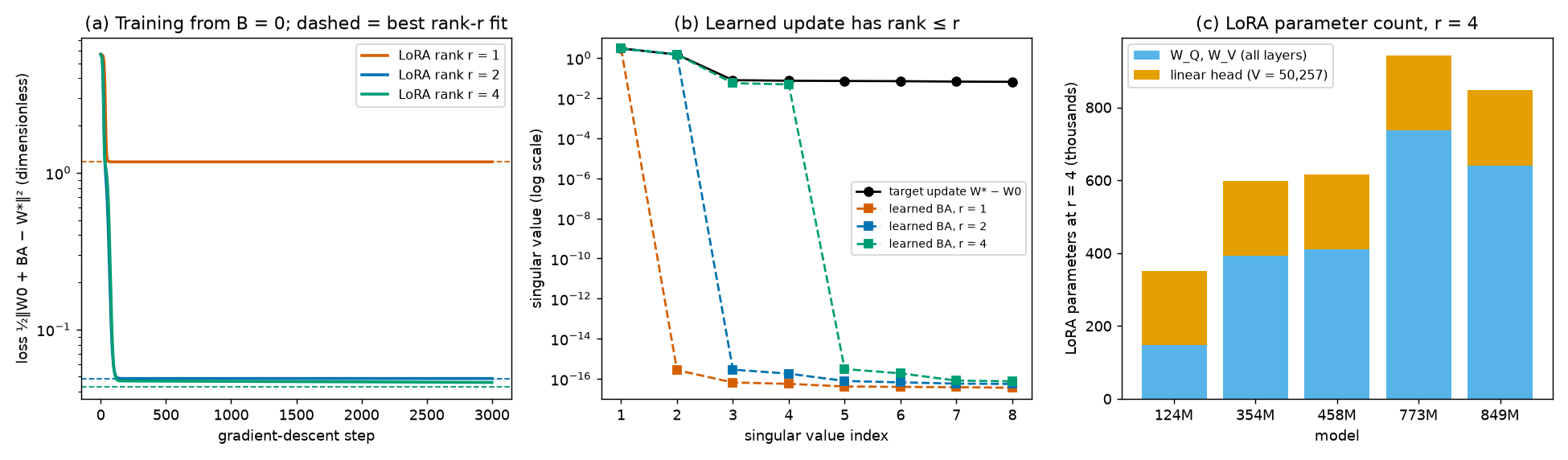
The head part barely grows (it depends on \(d_{\text{model}}\) only through \(r(V+d_{\text{model}})\), and \(V\) dominates), while the attention part grows with layers × width. Note that the 849M model has fewer LoRA numbers than the 773M model: it has fewer, wider layers.
Checking Hu et al.'s "10,000 times"¶
SOURCE: Hu et al. 2021, abstract; §4.2; §7.1 Hu et al. say LoRA cuts GPT-3 175B's trainable parameters by a factor of 10,000 (and GPU memory by 3); their main setting is \(r=4\) on \(W_q\) and \(W_v\) in all 96 layers, with width 12,288. PAPER §2, p. 3 The paper repeats the 10,000 and 3 figures.
MY EXPLANATION Using Hu et al.'s own count \(2\times(\text{number of adapted matrices})\times d_{\text{model}}\times r\): \(2\times192\times12{,}288\times4=18{,}874{,}368\) trainable numbers, and \(175\times10^9/18{,}874{,}368\approx9{,}272\) (output [4]). So "10,000 times" is a round-up of about 9,300 times. The memory figure cannot be checked from counts alone.
A toy you can watch: recovering a rank-2 change¶
To see LoRA learn, we need a problem whose answer we know. Take \(64\times64\) matrices (output [7]):
- a random start \(W_0\) (entries drawn from a normal distribution with variance \(1/64\));
- a target \(W^\star=W_0+(\text{a rank-2 change})+(\text{small noise})\). The rank-2 change is \(3\,u_1z_1^\top+1.5\,u_2z_2^\top\) with unit vectors \(u_1\perp u_2\) and \(z_1\perp z_2\); the noise has independent entries of standard deviation 0.005.
We train \(B\) and \(A\) to make \(W_0+BA\) close to \(W^\star\), with scale \(s=1\), by plain gradient descent (learning rate 0.05, 3,000 steps), starting from \(A\) Gaussian and \(B=0\). The loss is \(\tfrac12\lVert W_0+BA-W^\star\rVert_F^2\), where the Frobenius norm \(\lVert M\rVert_F\) is the norm of Chapter 8 applied to all entries of \(M\) at once: the square root of the sum of squared entries. Everything here is dimensionless.
The size of the true change is \(\lVert\cdot\rVert_F=3.3541\) and of the noise 0.3217. The dashed "best rank-\(r\)" level is the smallest loss any rank-\(r\) update can reach (computed from the singular values; see the deeper block below).
| \(r\) | start loss | final loss | best possible rank-\(r\) loss | error vs true change (relative) | rank of learned \(BA\) | numbers trained |
|---|---|---|---|---|---|---|
| 1 | 5.6908 | 1.174095 | 1.174095 | 0.4475 | 1 | 128 |
| 2 | 5.6908 | 0.048717 | 0.048717 | 0.0233 | 2 | 256 |
| 4 | 5.6908 | 0.045987 | 0.042895 | 0.0320 | 4 | 512 |
What the table shows:
- \(r=1\) is too small. It captures the larger pattern (strength 3) and must ignore the second (strength 1.5); the loss stays at 1.174095, exactly the best a rank-1 update can do, and the learned change is 45 % off.
- \(r=2\) recovers the change to within 2.33 %, using 256 numbers instead of the 4,096 entries of a dense \(64\times64\) matrix. What is left is the noise.
- \(r=4\) fits slightly better and recovers slightly worse. Its two extra directions slowly soak up noise (the noise's singular values are about 0.07), so its final loss is 7.2 % above its best level after 3,000 steps, and its error against the true change rises to 3.20 %. Extra rank bought fit to noise, not truth — the same trade-off the generalization bound is about.
Panel (b) of the figure shows the ranks directly: the learned updates have exactly 1, 2 and 4 singular values above rounding level (\(\approx10^{-16}\)).
Going deeper: singular values and the best rank-r approximation
MY EXPLANATION Singular value decomposition (SVD). Every real \(a\times b\) matrix \(M\) can be written as
with orthonormal vectors \(u_1,u_2,\dots\in\mathbb R^a\) and orthonormal \(z_1,z_2,\dots\in\mathbb R^b\). The numbers \(\sigma_i\) are the singular values. In words: every matrix is a sum of rank-1 patterns that do not overlap, sorted by strength. The rank is the number of nonzero \(\sigma_i\). (We skip the existence proof; it is standard linear algebra and follows from diagonalizing the symmetric matrix \(M^\top M\).) Our toy target was built in this form: \(\sigma_1=3\), \(\sigma_2=1.5\); the noise adds many small singular values, and the script finds \(3.006\), \(1.500\), \(0.079\), \(0.074\), \(0.072,\dots\) (output [7]).
Frobenius norm via singular values. Because the patterns are orthonormal, \(\lVert M\rVert_F^2=\sum_i\sigma_i^2\). (Expand \(\lVert M\rVert_F^2=\operatorname{trace}(M^\top M)\); cross terms contain \(u_i^\top u_j=0\) for \(i\neq j\), and each diagonal term gives \(\sigma_i^2\,(u_i^\top u_i)(z_i^\top z_i)=\sigma_i^2\).)
Eckart–Young theorem. Among all matrices \(X\) of rank at most \(r\), \(\lVert M-X\rVert_F\) is smallest for \(X=\sum_{i\le r}\sigma_iu_iz_i^\top\), and then \(\lVert M-X\rVert_F^2=\sum_{i>r}\sigma_i^2\).
Proof sketch. (1) Achievable: for this \(X\), \(M-X=\sum_{i>r}\sigma_iu_iz_i^\top\), whose squared norm is \(\sum_{i>r}\sigma_i^2\) by the previous paragraph. (2) Optimal: for any \(X\) of rank \(\le r\), the inequality \(\sigma_{i+r}(M)\le\sigma_i(M-X)\) holds for each \(i\) (Weyl's inequality for singular values, whose proof via the max–min characterization of \(\sigma_i\) we skip). Squaring and summing over \(i\) gives \(\lVert M-X\rVert_F^2\ge\sum_{i}\sigma_{i+r}(M)^2=\sum_{i>r}\sigma_i^2\). \(\blacksquare\)
So the best possible rank-\(r\) loss of the toy is \(\tfrac12\sum_{i>r}\sigma_i^2\) of \(W^\star-W_0\). For \(r=1\) that is dominated by \(\tfrac12\cdot1.5^2\); for \(r\ge2\) only noise remains. The script asserts that gradient descent from the standard initialization reaches this level for \(r=1,2\) to six decimals. (For this squared-error problem it is a known result, which we do not prove, that every local minimum of the factored loss is a global one, so gradient descent from a generic start ends at the best low-rank fit. It can get there very slowly along directions whose small singular values are nearly equal — exactly what \(r=4\) shows. For a real network no such guarantee exists.)
Going deeper¶
This section is a hub; the derivations sit in the collapsible blocks where they are needed.
- why \(BA\) is a sum of \(r\) outer products, and why an outer product has rank 1 (under "Low-rank update and the LoRA factors");
- the gradients \(\nabla_B\mathcal L=s\,GA^\top\), \(\nabla_A\mathcal L=s\,B^\top G\), the first LoRA step, and why \(A=B=0\) is a trap (under "Initialization");
- why, under Adam, the scale \(\alpha_{\text{LoRA}}/r\) acts as a learning-rate multiplier (under "The scaling factor");
- why the set of rank-\(\le r\) updates is a curved cone and not a subspace, bilinearity, and the \(r^2\) redundancy (under "LoRA for pretraining");
- singular values and the Eckart–Young theorem behind the toy's "best rank-\(r\)" line (under "Worked example").
Common misconceptions¶
- Misconception: LoRA makes the model smaller. — Actually: the network has exactly as many weights as before; \(W_0+sBA\) is a full \(a\times b\) matrix. LoRA shrinks the number of trained numbers, and therefore what must be stored given the seed for \(W_0\): 351,556 instead of 123,689,472 for GPT-2 small at \(r=4\).
- Misconception: Starting with \(B=0\) means LoRA starts with no learning signal. — Actually: the update is zero but the gradient with respect to \(B\) is not (0.3791 in output [6]); only the gradient with respect to \(A\) is zero, and only at the first step. Zero both factors and training is stuck forever (erratum E10's trap).
- Misconception: In this paper, LoRA fine-tunes a pretrained GPT-2. — Actually: the main experiments pretrain from random weights. \(W_0\) is random, and \(W_K\), \(W_O\), the MLPs and the layer norms stay random for the whole of training. (Only App. D fine-tunes, with SubLoRA at rank 8.)
- Misconception: A higher rank is always better. — Actually: it fits the training target better but can recover the true change worse: in the toy, \(r=4\) has relative error 0.0320 against 0.0233 for \(r=2\). And every extra number has to be paid for in the bound.
- Misconception: The \(r(a+b)\) trainable numbers are all independent degrees of freedom. — Actually: \((BM)(M^{-1}A)=BA\), so \(r^2\) of them are redundant (6,128 instead of 6,144 for a \(768\times768\) matrix at \(r=4\)).
- Misconception: Updates reachable by LoRA can be added and stay reachable. — Actually: two rank-1 updates sum to a rank-2 update (output [8]), which rank-1 LoRA cannot produce. The reachable set is curved.
Self-test¶
Q1. GPT-2 medium has 24 layers with \(d_{\text{model}}=1024\). Count the LoRA numbers at \(r=1\) (on \(W_Q\), \(W_V\) and the head, with \(V=50{,}257\)) and the head's share. Does the share change at \(r=4\)?
Answer
Attention: \(24\times2\times1\times(1024+1024)=98{,}304\). Head: \(1\times(50{,}257+1024)=51{,}281\). Total \(149{,}585\) (output [3]). Head share \(51{,}281/149{,}585=34.3\,\%\). At \(r=4\) both parts are multiplied by 4 (\(393{,}216\) and \(205{,}124\)), so the share is still 34.3 % (output [3]); it never depends on \(r\).
Q2. A colleague initializes both LoRA factors to zero "so that the model starts at \(W_0\)". Another initializes both randomly. What goes wrong in each case, and what does Hu et al.'s choice achieve?
Answer
Both zero: \(\nabla_B\mathcal L=s\,GA^\top=0\) and \(\nabla_A\mathcal L=s\,B^\top G=0\), so \((0,0)\) is a stationary point and gradient descent never moves (output [6]: loss 5.6908 before and after 500 steps). Both random: training can start, but \(BA\neq0\), so the model does not start at \(W_0\); in fine-tuning this damages the pretrained model before learning begins, and in the paper's setting it adds a random rank-\(r\) term to the starting point. Hu et al.'s choice (\(A\) random, \(B=0\)) gives \(\Delta W=0\) exactly and a nonzero gradient for \(B\). Either factor can be the zero one; what matters is that exactly one is.
Q3. Subspace training (Chapter 18) restricts \(\theta-\theta_0\) to a linear subspace. Is the set of updates reachable by LoRA on one matrix a linear subspace? Why does the answer matter to the paper?
Answer
No. The set is \(\{M:\operatorname{rank}M\le r\}\), which is closed under scaling but not under addition: two rank-1 matrices can sum to rank 2 (\(E_{11}+E_{22}=I\) for \(2\times2\); output [8]). The map from \((B,A)\) to \(BA\) is bilinear, not linear. The paper calls LoRA a nonlinear parameterization for this reason, and SubLoRA (Chapter 20) combines this curved set with a linear random subspace. The curvature is also why the starting point matters: at \(B=A=0\) the gradient vanishes (erratum E10).
Code for this chapter¶
Run it from the project root:
.venv/Scripts/python explainer/code/ch19_lora.py
Source: ch19_lora.py
"""Chapter 19 demo -- LoRA: low-rank adaptation.

Claims reproduced / checked (every number quoted in Chapter 19 is printed here):
  [1] One 768 x 768 attention matrix: a*b entries vs r*(a+b) LoRA numbers (r = 1, 4, 8).
  [2] GPT-2 small, LoRA on W_Q and W_V of all 12 layers and on the linear head (App. E, p. 16):
      12*2*r*(768+768) + r*(768+V); totals for r = 1 and r = 4; the head's share; the fraction of the
      123,689,472-parameter model (nanoGPT count, ch05_param_count.py). V = 50,257 [SOURCE: GPT-2
      tokenizer; never printed in the paper, erratum E36]; nanoGPT pads the vocabulary to 50,304
      [SOURCE: nanoGPT / authors' code], which is what the authors' code actually trains.
  [3] The same count for the paper's larger models (354M, 458M, 773M, 849M; shapes from ch05_param_count.py).
  [4] Hu et al. (2021): GPT-3 175B, r = 4 on W_q and W_v in 96 layers of width 12,288 -> trainable
      parameters and the "10,000 times" reduction [SOURCE: Hu et al. 2021, abstract, Sec. 4.2, 7.1].
  [5] The scaling factor alpha_LoRA / r with alpha_LoRA = 32 [PAPER App. E].
  [6] Initialization (Hu et al. Sec. 4.1): A Gaussian, B = 0 => Delta W = 0 exactly, grad wrt B nonzero,
      grad wrt A zero; with A = B = 0 both gradients vanish and training never moves (preview of
      erratum E10). Gradient formulas checked against torch autograd.
  [7] Low-rank recovery toy: 64 x 64 target W* = W0 + (rank-2 update) + noise, LoRA r = 1, 2, 4 trained
      by plain gradient descent from the standard init; compared with the best possible rank-r fit
      (Eckart-Young, via the SVD).
  [8] Non-closure: two rank-1 matrices sum (and average) to a rank-2 matrix.
  [9] Merging: (W0 + s BA) x equals W0 x + s B (A x) to rounding error.
 [10] Paper values used as forward pointers (Tables 1-2, p. 6-7), with log2 V recomputed.
Figure: explainer/docs/assets/fig/ch19_lora.png
Deterministic (numpy default_rng(0), torch.manual_seed(0)); CPU only; runs in a few seconds.
"""
from __future__ import annotations

import math
import sys
from pathlib import Path

import numpy as np
import matplotlib

matplotlib.use("Agg")
import matplotlib.pyplot as plt  # noqa: E402
import torch  # noqa: E402

HERE = Path(__file__).resolve().parent
sys.path.insert(0, str(HERE))
import pacbound  # noqa: E402

OUT_TXT = HERE / "outputs" / "ch19_lora.txt"
OUT_FIG = HERE.parent / "docs" / "assets" / "fig" / "ch19_lora.png"
V = pacbound.V_GPT2          # 50,257 [SOURCE: GPT-2 tokenizer]
V_PAD = 50304                # nanoGPT's padded vocabulary [SOURCE: nanoGPT / authors' code]
ALPHA_LORA = 32              # [PAPER App. E, p. 16] "LoRA alpha value of 32"

_lines: list[str] = []


def out(s: str = "") -> None:
    print(s)
    _lines.append(s)


def lora_numbers(a: int, b: int, r: int) -> int:
    """Entries of B (a x r) plus A (r x b)."""
    return r * (a + b)


def gpt2_lora(n_layer: int, d: int, r: int, vocab: int = V) -> tuple[int, int, int]:
    """LoRA on W_Q and W_V (d x d each) in every layer and on the head (d -> vocab).
    Returns (q,v part, head part, total)."""
    qv = n_layer * 2 * lora_numbers(d, d, r)
    head = lora_numbers(vocab, d, r)
    return qv, head, qv + head


def rank(M: np.ndarray) -> int:
    return int(np.linalg.matrix_rank(M))


# --------------------------------------------------------------------------- [1]
out("Chapter 19 -- LoRA: low-rank adaptation (ch19_lora.py)")
a = b = 768
full = a * b
out(f"[1] one 768 x 768 matrix (W_Q or W_V of GPT-2 small): a*b = {full:,} entries")
for r in (1, 4, 8):
    n = lora_numbers(a, b, r)
    out(f"    r = {r}: B is 768x{r}, A is {r}x768 -> r(a+b) = {n:,} numbers  ({full / n:.1f}x fewer)")
assert lora_numbers(768, 768, 4) == 6144 and full // 6144 == 96
out(f"    redundancy: BA = (BM)(M^-1 A) for any invertible r x r M, so rank-r matrices form a set of dimension"
    f" r(a+b) - r^2 = {lora_numbers(a, b, 4) - 16:,} (r = 4)")

# --------------------------------------------------------------------------- [2]
base_small = pacbound.gpt2_params(12, 768)     # 123,689,472 (nanoGPT count, ch05)
out(f"[2] GPT-2 small (12 layers, d = 768, V = {V:,} [SOURCE: GPT-2 tokenizer]); model = {base_small:,} params")
out("    r   q,v: 12*2*r*1536   head: r*(768+V)   total      head share   % of model")
small = {}
for r in (1, 4, 8):
    qv, head, tot = gpt2_lora(12, 768, r)
    small[r] = (qv, head, tot)
    out(f"    {r}   {qv:>14,}   {head:>14,}   {tot:>9,}   {100 * head / tot:6.2f} %    {100 * tot / base_small:.3f} %")
assert small[4] == (147456, 204100, 351556) and small[1][2] == 87889
qv4p, head4p, tot4p = gpt2_lora(12, 768, 4, V_PAD)
qv1p, head1p, tot1p = gpt2_lora(12, 768, 1, V_PAD)
out(f"    with nanoGPT's padded vocabulary 50,304 (what the authors' code trains): r = 1 -> {tot1p:,};"
    f" r = 4 -> {tot4p:,} (head {head4p:,}); difference (50,304 - 50,257) x r = {tot1p - small[1][2]} at r = 1,"
    f" {tot4p - small[4][2]} at r = 4")
out(f"    the head's long side V is {V / 768:.1f} times d_model = 768")
out(f"    r = 4: dense W_Q and W_V of 12 layers would be {12 * 2 * full:,} numbers; dense head {768 * V:,}")
out(f"    ratio model / LoRA(r=4) = {base_small / small[4][2]:.0f}x;  model / LoRA(r=1) = {base_small / small[1][2]:.0f}x")

# --------------------------------------------------------------------------- [3]
out("[3] larger models of the paper (shapes from ch05_param_count.py; 458M and 849M inferred there)")
out("    model  layers x d     r=1 total   r=4: q,v      head       total     head share  % of model")
SIZES = [("124M", 12, 768), ("354M", 24, 1024), ("458M", 20, 1280), ("773M", 36, 1280), ("849M", 25, 1600)]
bars = []
for name, nl, d in SIZES:
    base = pacbound.gpt2_params(nl, d)
    t1 = gpt2_lora(nl, d, 1)[2]
    qv, head, tot = gpt2_lora(nl, d, 4)
    t8 = gpt2_lora(nl, d, 8)[2]
    bars.append((name, qv, head))
    out(f"    {name}   {nl:>2} x {d:<5}  {t1:>10,}   {qv:>9,}  {head:>9,}  {tot:>9,}   {100 * head / tot:5.1f} %"
        f"     {100 * tot / base:.3f} %   (r=8: {t8:,})")

# --------------------------------------------------------------------------- [4]
n_layers3, d3, r3 = 96, 12288, 4
lora3 = 2 * (n_layers3 * 2) * d3 * r3          # |Theta| = 2 * L_LoRA * d_model * r, L_LoRA = 192 matrices
out("[4] Hu et al. (2021): GPT-3 175B, r = 4 on W_q and W_v of 96 layers, d_model = 12,288")
out(f"    trainable = 2 x 192 matrices x 12,288 x 4 = {lora3:,};  175e9 / that = {175e9 / lora3:,.0f}x"
    f"  (abstract: '10,000 times')")
out(f"    same budget with r = 8 on one matrix type: 2 x 96 x 12,288 x 8 = {2 * 96 * d3 * 8:,}")

# --------------------------------------------------------------------------- [5]
out(f"[5] scaling s = alpha_LoRA / r with alpha_LoRA = {ALPHA_LORA} [PAPER App. E]: "
    + ", ".join(f"r = {r} -> s = {ALPHA_LORA / r:g}" for r in (1, 4, 8)))

# --------------------------------------------------------------------------- [6]
rng = np.random.default_rng(0)
A_, B_ = 64, 64
W0 = rng.normal(0.0, 1.0 / math.sqrt(B_), size=(A_, B_))             # random "pretraining" start
u, _ = np.linalg.qr(rng.normal(size=(A_, 2)))
v, _ = np.linalg.qr(rng.normal(size=(B_, 2)))
sig_true = np.array([3.0, 1.5])
D_true = (u * sig_true) @ v.T                                          # exact rank-2 update
noise = rng.normal(0.0, 0.005, size=(A_, B_))
W_star = W0 + D_true + noise
T = W_star - W0                                                        # what the update must supply


def loss_grads(Bm, Am, s=1.0):
    """L = 0.5 ||W0 + s BA - W*||_F^2 ; G = dL/dW ; dL/dB = s G A^T ; dL/dA = s B^T G."""
    G = s * (Bm @ Am) - T
    return 0.5 * float(np.sum(G * G)), s * G @ Am.T, s * Bm.T @ G


r = 2
A0 = rng.normal(0.0, 1.0 / math.sqrt(B_), size=(r, B_))   # Gaussian A (Hu et al. Sec. 4.1)
B0 = np.zeros((A_, r))                                     # B = 0
L0, gB, gA = loss_grads(B0, A0)
out("[6] initialization on the 64 x 64 toy (r = 2, s = 1):")
out(f"    A Gaussian, B = 0:  ||Delta W||_F = {np.linalg.norm(B0 @ A0):.1f}   loss = {L0:.4f}   "
    f"||dL/dB||_F = {np.linalg.norm(gB):.4f}   ||dL/dA||_F = {np.linalg.norm(gA):.1f}")
# torch autograd cross-check of the formulas
tB = torch.tensor(B0 + 0.1 * rng.normal(size=B0.shape), requires_grad=True)
tA = torch.tensor(A0, requires_grad=True)
tl = 0.5 * ((tB @ tA - torch.tensor(T)) ** 2).sum()
tl.backward()
_, gB2, gA2 = loss_grads(tB.detach().numpy(), A0)
err_ad = max(np.abs(tB.grad.numpy() - gB2).max(), np.abs(tA.grad.numpy() - gA2).max())
out(f"    formulas dL/dB = s G A^T, dL/dA = s B^T G match torch autograd (generic point): max diff {err_ad:.1e}")
assert err_ad < 1e-10
Bz, Az = np.zeros((A_, r)), np.zeros((r, B_))
Lz, gBz, gAz = loss_grads(Bz, Az)
for _ in range(500):
    _, gb, ga = loss_grads(Bz, Az)
    Bz, Az = Bz - 0.1 * gb, Az - 0.1 * ga
Lz_end = loss_grads(Bz, Az)[0]
out(f"    A = B = 0:          ||dL/dB||_F = {np.linalg.norm(gBz):.1f}   ||dL/dA||_F = {np.linalg.norm(gAz):.1f}"
    f"   loss {Lz:.4f} -> {Lz_end:.4f} after 500 GD steps (stuck; cf. erratum E10)")
assert np.linalg.norm(B0 @ A0) == 0.0 and np.linalg.norm(gB) > 0 and np.linalg.norm(gA) == 0.0
assert Lz_end == Lz

# --------------------------------------------------------------------------- [7]
sv_T = np.linalg.svd(T, compute_uv=False)
out("[7] recovery toy: W* = W0 + rank-2 update (singular values 3, 1.5) + N(0, 0.005^2) noise, 64 x 64")
out(f"    ||true update||_F = {np.linalg.norm(D_true):.4f}   ||noise||_F = {np.linalg.norm(noise):.4f}   "
    f"top singular values of W* - W0: {', '.join(f'{x:.3f}' for x in sv_T[:5])}")
out("    plain GD, lr 0.05, 3000 steps, s = 1, A ~ N(0, 1/64) and B = 0 at the start")
out("    r   start loss   final loss   best rank-r loss   rel. error vs true update   numerical rank   numbers")
curves, svs = {}, {}
for r in (1, 2, 4):
    rr = np.random.default_rng(100 + r)
    Am = rr.normal(0.0, 1.0 / math.sqrt(B_), size=(r, B_))
    Bm = np.zeros((A_, r))
    hist = []
    for step in range(3000):
        L, gb, ga = loss_grads(Bm, Am)
        hist.append(L)
        Bm, Am = Bm - 0.05 * gb, Am - 0.05 * ga
    Lf = loss_grads(Bm, Am)[0]
    hist.append(Lf)
    best = 0.5 * float(np.sum(sv_T[r:] ** 2))                    # Eckart-Young optimum
    dW = Bm @ Am
    rel = np.linalg.norm(dW - D_true) / np.linalg.norm(D_true)
    s_dW = np.linalg.svd(dW, compute_uv=False)
    nrank = int(np.sum(s_dW > 1e-8 * s_dW[0]))
    curves[r], svs[r] = np.array(hist), s_dW
    out(f"    {r}   {hist[0]:9.4f}   {Lf:10.6f}   {best:14.6f}     {rel:22.4f}      {nrank:>6}"
        f"        {lora_numbers(A_, B_, r):>5}")
    if r <= 2:
        assert abs(Lf - best) < 1e-6 * max(1.0, best) + 1e-6, (r, Lf, best)
    else:
        assert best <= Lf < 1.1 * best and Lf < curves[2][-1], (r, Lf, best)
    if r >= 2:
        assert rel < 0.05
gap4 = curves[4][-1] / (0.5 * float(np.sum(sv_T[4:] ** 2))) - 1
out(f"    dense 64 x 64 would need {A_ * B_:,} numbers. r = 1, 2 reach the best rank-r loss; r = 4 is {100 * gap4:.1f} %"
    f" above it,")
out("    because its 2 extra directions slowly fit noise (singular values ~0.07) -- and its error vs the true update grows")

# --------------------------------------------------------------------------- [8]
out("[8] non-closure under addition")
E1 = np.array([[1.0, 0.0], [0.0, 0.0]])
E2 = np.array([[0.0, 0.0], [0.0, 1.0]])
out(f"    [[1,0],[0,0]] (rank {rank(E1)}) + [[0,0],[0,1]] (rank {rank(E2)}) = identity (rank {rank(E1 + E2)})")
rr = np.random.default_rng(7)
R1 = np.outer(rr.normal(size=64), rr.normal(size=64))
R2 = np.outer(rr.normal(size=64), rr.normal(size=64))
out(f"    random 64 x 64: rank(b1 a1) = {rank(R1)}, rank(b2 a2) = {rank(R2)}, rank(sum) = {rank(R1 + R2)}, "
    f"rank(average) = {rank(0.5 * (R1 + R2))}, rank(-3 x b1 a1) = {rank(-3 * R1)}")
assert rank(R1 + R2) == 2 and rank(E1 + E2) == 2

# --------------------------------------------------------------------------- [9]
rr = np.random.default_rng(11)
Bm, Am, x = rr.normal(size=(64, 4)), rr.normal(size=(4, 64)), rr.normal(size=64)
s = ALPHA_LORA / 4
y_branch = W0 @ x + s * (Bm @ (Am @ x))
y_merged = (W0 + s * Bm @ Am) @ x
out(f"[9] merge check (r = 4, s = 8): max |(W0 + sBA)x - (W0 x + sB(Ax))| = {np.abs(y_branch - y_merged).max():.1e}")
assert np.abs(y_branch - y_merged).max() < 1e-10

# --------------------------------------------------------------------------- [10]
out("[10] paper values used as forward pointers [PAPER Tables 1-2, p. 6-7]")
out("     BPD bound: SubLoRA 12.12, LoRA only 13.09, original 70.76; validation BPD: LoRA only 11.21, original 4.35")
out(f"     random-guess BPD = log2 V = log2 {V:,} = {math.log2(V):.3f} bits/token (paper prints 15.62)")
assert abs(math.log2(V) - 15.62) < 0.005

OUT_TXT.parent.mkdir(parents=True, exist_ok=True)
OUT_TXT.write_text("\n".join(_lines) + "\n", encoding="utf-8")

# --------------------------------------------------------------------------- figure
fig, axes = plt.subplots(1, 3, figsize=(15, 4.4))
cols = {1: "#D55E00", 2: "#0072B2", 4: "#009E73"}
ax = axes[0]
for r in (1, 2, 4):
    ax.semilogy(curves[r], color=cols[r], lw=2, label=f"LoRA rank r = {r}")
    best = 0.5 * float(np.sum(sv_T[r:] ** 2))
    ax.axhline(best, color=cols[r], ls="--", lw=1)
ax.set_xlabel("gradient-descent step")
ax.set_ylabel("loss ½‖W0 + BA − W*‖² (dimensionless)")
ax.set_title("(a) Training from B = 0; dashed = best rank-r fit")
ax.legend(fontsize=9)
ax = axes[1]
k = np.arange(1, 9)
ax.semilogy(k, sv_T[:8], "o-", color="#000000", label="target update W* − W0")
for r in (1, 2, 4):
    sv = np.maximum(svs[r][:8], 1e-17)
    ax.semilogy(k, sv, "s--", color=cols[r], ms=5, label=f"learned BA, r = {r}")
ax.set_xlabel("singular value index")
ax.set_ylabel("singular value (log scale)")
ax.set_ylim(1e-17, 10)
ax.set_title("(b) Learned update has rank ≤ r")
ax.legend(fontsize=8)
ax = axes[2]
names = [bb[0] for bb in bars]
qvs = np.array([bb[1] for bb in bars]) / 1e3
heads = np.array([bb[2] for bb in bars]) / 1e3
ax.bar(names, qvs, color="#56B4E9", label="W_Q, W_V (all layers)")
ax.bar(names, heads, bottom=qvs, color="#E69F00", label="linear head (V = 50,257)")
ax.set_ylabel("LoRA parameters at r = 4 (thousands)")
ax.set_xlabel("model")
ax.set_title("(c) LoRA parameter count, r = 4")
ax.legend(fontsize=9)
fig.tight_layout()
OUT_FIG.parent.mkdir(parents=True, exist_ok=True)
fig.savefig(OUT_FIG, dpi=130)
print(f"figure: {OUT_FIG.relative_to(HERE.parent.parent)}")
print("All assertions passed.")
Output:
Chapter 19 -- LoRA: low-rank adaptation (ch19_lora.py)
[1] one 768 x 768 matrix (W_Q or W_V of GPT-2 small): a*b = 589,824 entries
    r = 1: B is 768x1, A is 1x768 -> r(a+b) = 1,536 numbers  (384.0x fewer)
    r = 4: B is 768x4, A is 4x768 -> r(a+b) = 6,144 numbers  (96.0x fewer)
    r = 8: B is 768x8, A is 8x768 -> r(a+b) = 12,288 numbers  (48.0x fewer)
    redundancy: BA = (BM)(M^-1 A) for any invertible r x r M, so rank-r matrices form a set of dimension r(a+b) - r^2 = 6,128 (r = 4)
[2] GPT-2 small (12 layers, d = 768, V = 50,257 [SOURCE: GPT-2 tokenizer]); model = 123,689,472 params
    r   q,v: 12*2*r*1536   head: r*(768+V)   total      head share   % of model
    1           36,864           51,025      87,889    58.06 %    0.071 %
    4          147,456          204,100     351,556    58.06 %    0.284 %
    8          294,912          408,200     703,112    58.06 %    0.568 %
    with nanoGPT's padded vocabulary 50,304 (what the authors' code trains): r = 1 -> 87,936; r = 4 -> 351,744 (head 204,288); difference (50,304 - 50,257) x r = 47 at r = 1, 188 at r = 4
    the head's long side V is 65.4 times d_model = 768
    r = 4: dense W_Q and W_V of 12 layers would be 14,155,776 numbers; dense head 38,597,376
    ratio model / LoRA(r=4) = 352x;  model / LoRA(r=1) = 1407x
[3] larger models of the paper (shapes from ch05_param_count.py; 458M and 849M inferred there)
    model  layers x d     r=1 total   r=4: q,v      head       total     head share  % of model
    124M   12 x 768        87,889     147,456    204,100    351,556    58.1 %     0.284 %   (r=8: 703,112)
    354M   24 x 1024      149,585     393,216    205,124    598,340    34.3 %     0.169 %   (r=8: 1,196,680)
    458M   20 x 1280      153,937     409,600    206,148    615,748    33.5 %     0.134 %   (r=8: 1,231,496)
    773M   36 x 1280      235,857     737,280    206,148    943,428    21.9 %     0.122 %   (r=8: 1,886,856)
    849M   25 x 1600      211,857     640,000    207,428    847,428    24.5 %     0.100 %   (r=8: 1,694,856)
[4] Hu et al. (2021): GPT-3 175B, r = 4 on W_q and W_v of 96 layers, d_model = 12,288
    trainable = 2 x 192 matrices x 12,288 x 4 = 18,874,368;  175e9 / that = 9,272x  (abstract: '10,000 times')
    same budget with r = 8 on one matrix type: 2 x 96 x 12,288 x 8 = 18,874,368
[5] scaling s = alpha_LoRA / r with alpha_LoRA = 32 [PAPER App. E]: r = 1 -> s = 32, r = 4 -> s = 8, r = 8 -> s = 4
[6] initialization on the 64 x 64 toy (r = 2, s = 1):
    A Gaussian, B = 0:  ||Delta W||_F = 0.0   loss = 5.6908   ||dL/dB||_F = 0.3791   ||dL/dA||_F = 0.0
    formulas dL/dB = s G A^T, dL/dA = s B^T G match torch autograd (generic point): max diff 1.1e-16
    A = B = 0:          ||dL/dB||_F = 0.0   ||dL/dA||_F = 0.0   loss 5.6908 -> 5.6908 after 500 GD steps (stuck; cf. erratum E10)
[7] recovery toy: W* = W0 + rank-2 update (singular values 3, 1.5) + N(0, 0.005^2) noise, 64 x 64
    ||true update||_F = 3.3541   ||noise||_F = 0.3217   top singular values of W* - W0: 3.006, 1.500, 0.079, 0.074, 0.072
    plain GD, lr 0.05, 3000 steps, s = 1, A ~ N(0, 1/64) and B = 0 at the start
    r   start loss   final loss   best rank-r loss   rel. error vs true update   numerical rank   numbers
    1      5.6908     1.174095         1.174095                     0.4475           1          128
    2      5.6908     0.048717         0.048717                     0.0233           2          256
    4      5.6908     0.045987         0.042895                     0.0320           4          512
    dense 64 x 64 would need 4,096 numbers. r = 1, 2 reach the best rank-r loss; r = 4 is 7.2 % above it,
    because its 2 extra directions slowly fit noise (singular values ~0.07) -- and its error vs the true update grows
[8] non-closure under addition
    [[1,0],[0,0]] (rank 1) + [[0,0],[0,1]] (rank 1) = identity (rank 2)
    random 64 x 64: rank(b1 a1) = 1, rank(b2 a2) = 1, rank(sum) = 2, rank(average) = 2, rank(-3 x b1 a1) = 1
[9] merge check (r = 4, s = 8): max |(W0 + sBA)x - (W0 x + sB(Ax))| = 5.3e-14
[10] paper values used as forward pointers [PAPER Tables 1-2, p. 6-7]
     BPD bound: SubLoRA 12.12, LoRA only 13.09, original 70.76; validation BPD: LoRA only 11.21, original 4.35
     random-guess BPD = log2 V = log2 50,257 = 15.617 bits/token (paper prints 15.62)