22. Entropy and arithmetic coding

Where this fits

Prerequisites: Chapter 3 (\(\log_2\), bits, surprisal, \(\ln x \le x - 1\), the 8,192-bit kilobyte), Chapter 12 (codes, prefix-free codes, the Kraft inequality and its converse, the length header). We also use the chain rule of probability from Chapter 4, negative log-likelihood and cross-entropy from Chapter 6, and the quantized weights of Chapter 21. Used later by: Chapter 24 (Algorithm 1's GET_COMPRESSED_SIZE), Chapter 26 (the "compressed dataset size" of Figure 3) and Chapter 28 (mini replication). Purpose: explain how the paper turns its quantized weights into a number of bits \(C(h)\), why that number is close to \(d\) times the entropy, and why no code can do much better.

The problem this chapter solves

Everything in this section is MY EXPLANATION unless tagged.

The bound of the paper charges a model for its compressed size \(C(h)\), in bits (Chapter 12, Chapter 14). Every bit saved makes the bound tighter. So the paper needs a way to write its trained model down in as few bits as possible.

Here is what has to be written down. A quick reminder from Chapter 21: after quantization, the trainable part of the model is a list \(\hat w\) of \(d\) numbers, and each of them equals one of \(L_q\) allowed values (the quantization levels, stored in a short table called the codebook). So \(\hat w\) is really a list of \(d\) symbols, each taken from an "alphabet" of \(L_q\) possibilities. Everything else in the model (the architecture, the random starting point, the random projection) is regenerated from fixed seeds and costs nothing (Chapter 20).

PAPER §6.1, p. 7 The paper expresses \(w\) in this quantization and encodes it with arithmetic coding to get the compressed size of the model. The bits that name the chosen hyperparameters are added on top.

PAPER App. C, Algorithm 1 lines 16–21, p. 15; App. E, p. 16 The function GET_COMPRESSED_SIZE first counts how often each level occurs in \(\hat w\), then runs arithmetic coding with those counts. Appendix E says the bitstream is produced "from the empirical probabilities over the quantization bins", that is, from the fractions of weights that fall on each level. Appendix C adds that arithmetic coding exploits the fact that some levels are more frequent than others.

MY EXPLANATION The simplest code would give every weight the same number of bits. With \(L_q = 11\) levels that is \(\lceil \log_2 11\rceil = 4\) bits per weight (Chapter 3). For \(d = 50{,}000\) weights that is 200,000 bits, or 24.414 KB.

[PAPER Fig. 2 left, p. 5; read exactly from the PDF by fig_extract.py] The model behind the paper's best bound has \(d = 50{,}000\) and a compressed size of 16.5325 KB. With 1 KB = 8,192 bits (erratum E35) that is 135,434 bits, or 2.709 bits per weight.

MY EXPLANATION So the paper spends 32.3 % less than the 4-bit code. This chapter answers three questions:

1. What is the smallest average number of bits per symbol that any code can reach? Answer: the entropy of the symbol frequencies. Proving this needs Gibbs' inequality.
2. How does one get there in practice? Answer: arithmetic coding, which pays at most 2 bits more than the ideal for the whole message, not per symbol.
3. What else must be stored so that a decoder can undo the code? Answer: the codebook and the symbol counts (a small header), and the length header of Chapter 12.

The same machinery explains a sentence of §7.1: a language model plus arithmetic coding compresses text to about its negative log-likelihood in bits.

Intuition (and where the analogy breaks)

Everything in this section is MY EXPLANATION.

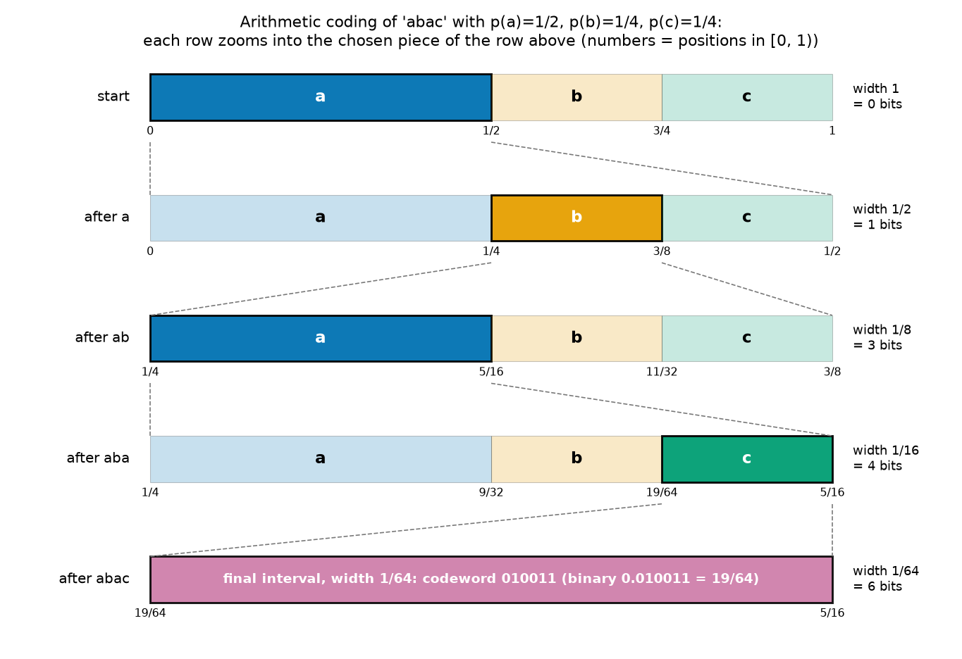
Zooming into a ruler. Take a ruler from 0 to 1. Mark it into segments, one per symbol, with lengths equal to the symbol probabilities. With \(p(a) = 1/2\), \(p(b) = 1/4\), \(p(c) = 1/4\), the segment of \(a\) covers the first half, \(b\) the next quarter and \(c\) the last quarter.

To send the message "abac", zoom into the segment of the first letter, \(a\). Mark that piece again in the same proportions and zoom into the segment of the second letter, \(b\). Repeat for every letter. Each step shrinks the piece by the probability of the letter: by 1/2 for \(a\), by 1/4 for \(b\). After four letters the piece has width \(\tfrac12\cdot\tfrac14\cdot\tfrac12\cdot\tfrac14 = \tfrac1{64}\).

Now you only have to tell the receiver an address on the ruler that is precise enough to land inside that final tiny piece. The receiver repeats the zooming: whichever segment contains the address must be the letter that was sent.

How precise must the address be? Each binary digit of an address halves the uncertainty about where it points. A piece of width \(1/64 = 2^{-6}\) needs about 6 binary digits. In general a piece of width \(W\) needs about \(\log_2(1/W)\) bits.

And \(\log_2(1/W)\) is the sum of the surprisals of the letters, because the width is a product of probabilities and a logarithm turns products into sums (Chapter 3). Likely letters shrink the piece only a little and cost a fraction of a bit. Rare letters shrink it a lot and cost many bits. Nothing is rounded letter by letter, so a letter of probability 0.95 really costs only \(\log_2(1/0.95) = 0.074\) bits.

Where it breaks.

• The exact version needs ever finer fractions: after the 50,000 symbols of Step 5 below, the final width is about \(2^{-140{,}088}\), so the endpoints need about 140,088 binary digits. Real coders use fixed-size integers (for example 32 bits) and "renormalize": they write out the leading digits that can no longer change and zoom the integer range back up. This costs a tiny amount of extra length (a Going-deeper block bounds it). The exact-fraction version here is for understanding.
• A ruler's marks are fixed. Here the segment lengths follow the probabilities, and with a language model they change at every step, because the probabilities of the next symbol depend on the earlier ones.
• "An address inside the piece" is not quite enough. The address must be such that every longer address beginning with the same digits still lands inside. Otherwise one codeword could be the beginning of another, and the code would not be prefix-free (Chapter 12). This costs at most one extra bit.
• A ruler reading does not say when to stop. The receiver must also be told how many letters to decode.

Precise definition

Everything in this section is MY EXPLANATION (standard information theory) unless tagged.

Sources, symbols and messages

• An alphabet here is a finite set of \(L\) symbols, numbered \(1, \dots, L\). For the paper's weights, \(L = L_q\) and symbol \(k\) means "this weight equals the \(k\)-th quantization level".
• A distribution on the alphabet is a list \(p = (p_1, \dots, p_L)\) of numbers \(p_k \ge 0\) with \(\sum_k p_k = 1\) (Chapter 1).
• A message of length \(n\) is a sequence \(x = (x_1, \dots, x_n)\) of symbols.
• An i.i.d. source with distribution \(p\) produces a message whose symbols are independent and each equal to \(k\) with probability \(p_k\). Then \(\Pr[X = x] = p_{x_1} p_{x_2}\cdots p_{x_n}\); the probability is over the random symbols, and \(p\) is fixed.

Entropy

The entropy of a distribution \(p\) is

\[ H(p) = -\sum_{k=1}^{L} p_k \log_2 p_k = \sum_{k=1}^{L} p_k \log_2\frac{1}{p_k} \quad \text{bits per symbol}, \]

with the convention that a term with \(p_k = 0\) counts as 0. (This is the limit of \(p\log_2(1/p)\) as \(p \to 0\); it says that an impossible symbol contributes nothing.)

In words: \(\log_2(1/p_k)\) is the surprisal of symbol \(k\) (Chapter 3), and \(H(p)\) is the average surprisal, weighting each symbol by how often it occurs.

Three facts, proved in the next Going-deeper blocks:

• \(H(p) \ge 0\), with \(H(p) = 0\) exactly when one symbol has probability 1 (no surprise at all).
• \(H(p) \le \log_2 L\), with equality exactly when all \(L\) symbols are equally likely. For \(L_q = 11\) levels the maximum is \(\log_2 11 = 3.4594\) bits; for 17 levels it is \(\log_2 17 = 4.0875\) bits.
• For a message of \(n\) independent symbols the entropies add: the whole message has entropy \(n H(p)\).

Examples (script block [2]): \(H(1/2, 1/4, 1/4) = 1.5000\) bits; \(H(0.6, 0.3, 0.1) = 1.2955\) bits; \(H(0.95, 0.05) = 0.2864\) bits.

Gibbs' inequality

Let \(p\) be a distribution and let \(q = (q_1, \dots, q_L)\) be any numbers with \(q_k \ge 0\) and \(\sum_k q_k \le 1\). Then

\[ \sum_{k:\,p_k>0} p_k \log_2 \frac{p_k}{q_k} \;\ge\; 0 , \]

with equality only when \(q = p\). The left side is called the relative entropy or Kullback–Leibler (KL) divergence of \(p\) from \(q\). It is \(+\infty\) if some \(q_k = 0\) while \(p_k > 0\).

An equivalent form: the cross-entropy \(-\sum_k p_k \log_2 q_k\), defined in Chapter 6 as the average surprisal when the data follow \(p\) but the probabilities used are \(q\), is never smaller than \(H(p)\). Using the wrong probabilities always costs extra bits on average.

Going deeper: proof of Gibbs' inequality

MY EXPLANATION Setting. \(p\) is a distribution on \(\{1,\dots,L\}\); \(q_k \ge 0\) with \(\sum_k q_k \le 1\). Let \(S = \{k : p_k > 0\}\) be the symbols that can occur. Everything is fixed; nothing is random.

Case 1: some \(k \in S\) has \(q_k = 0\). Then that term is \(p_k\log_2(p_k/0) = +\infty\), and the sum is \(+\infty \ge 0\). (Using such a \(q\) for coding would mean a symbol that can occur gets no codeword at all.)

Case 2: \(q_k > 0\) for every \(k \in S\). Multiply the sum by \(-\ln 2 < 0\) and use \(\log_2 y = \ln y / \ln 2\):

\[ -\ln 2 \sum_{k\in S} p_k \log_2\frac{p_k}{q_k} = \sum_{k \in S} p_k \ln\frac{q_k}{p_k} . \]

Apply \(\ln y \le y - 1\) (Chapter 3) with \(y = q_k/p_k > 0\) to every term:

\[ \begin{aligned} \sum_{k \in S} p_k \ln\frac{q_k}{p_k} &\le \sum_{k \in S} p_k\Big(\frac{q_k}{p_k} - 1\Big) \\ &= \sum_{k\in S} q_k - \sum_{k \in S} p_k \\ &= \sum_{k\in S} q_k - 1 \;\le\; \sum_{k=1}^{L} q_k - 1 \;\le\; 0 . \end{aligned} \]

The step \(\sum_{k\in S} p_k = 1\) holds because the symbols outside \(S\) have \(p_k = 0\). So \(-\ln 2 \cdot (\text{our sum}) \le 0\), and dividing by \(-\ln 2\) flips the inequality: the sum is \(\ge 0\). ∎

Equality. All three inequalities must be equalities. The first needs \(\ln y = y - 1\) in every term, which happens only at \(y = 1\), so \(q_k = p_k\) for all \(k \in S\). The last two need \(\sum_k q_k = 1\) and no weight of \(q\) outside \(S\). Together: \(q = p\). Conversely \(q = p\) gives \(\log_2 1 = 0\) in every term. ∎

Cross-entropy form. Splitting the logarithm, \(\sum_{S} p_k\log_2(p_k/q_k) = -\sum_S p_k\log_2 q_k - H(p)\), so the inequality says \(-\sum_k p_k\log_2 q_k \ge H(p)\). Units: every term is in bits, because every logarithm is base 2.

Going deeper: entropy lies between 0 and log2 L, and adds over independent symbols

MY EXPLANATION Lower bound. For \(0 < p_k \le 1\) we have \(\log_2(1/p_k) \ge 0\), so every term \(p_k\log_2(1/p_k)\) is \(\ge 0\), and so is their sum. The sum is 0 only if every term is 0, that is, every \(p_k\) is 0 or 1. Since the \(p_k\) add up to 1, exactly one of them is 1.

Upper bound. Apply Gibbs with the uniform weights \(q_k = 1/L\) (they add up to 1):

\[ 0 \le \sum_{k:\,p_k>0} p_k\log_2\frac{p_k}{1/L} = \sum_{k:\,p_k>0} p_k \log_2 p_k + \log_2 L \sum_{k:\,p_k>0} p_k = -H(p) + \log_2 L . \]

So \(H(p) \le \log_2 L\), with equality only when \(p\) equals the uniform distribution.

Additivity. Let a message of \(n\) symbols come from an i.i.d. source, so \(\Pr[X = x] = \prod_i p_{x_i}\). Its entropy, as a distribution over the \(L^n\) possible messages, is

\[ \begin{aligned} H(p^{\otimes n}) &= -\sum_{x} \Big(\prod_{j} p_{x_j}\Big)\log_2 \prod_{i} p_{x_i} = -\sum_{i=1}^{n} \sum_{x} \Big(\prod_{j} p_{x_j}\Big)\log_2 p_{x_i} \\ &= -\sum_{i=1}^{n} \sum_{k=1}^{L} p_k \log_2 p_k = n\,H(p) . \end{aligned} \]

The middle step uses the product rule of logarithms. The last step sums out all positions except \(i\): for fixed \(x_i = k\) the other factors add up to \(\big(\sum_{k'} p_{k'}\big)^{n-1} = 1\). Here \(p^{\otimes n}\) is our name for the distribution of the whole message.

Shannon's source-coding bound

Suppose each symbol \(k\) gets its own codeword of length \(\ell_k\) bits, and the code is prefix-free (Chapter 12). The expected code length is \(\sum_k p_k \ell_k\) bits per symbol. Then:

• Lower bound (Shannon). For every prefix-free code, \(\sum_k p_k \ell_k \ge H(p)\). By McMillan's theorem (Chapter 12) the same holds for every uniquely decodable code. Equality needs \(\ell_k = \log_2(1/p_k)\) for every symbol, which is possible only if every \(p_k\) is a power of 1/2.
• Achievability within 1 bit. The lengths \(\ell_k = \lceil \log_2(1/p_k)\rceil\) satisfy the Kraft inequality, so by the converse of Kraft a prefix-free code with these lengths exists. It is called a Shannon code, and its expected length is less than \(H(p) + 1\).

The same two statements apply to a whole message treated as one big "symbol": a message of \(n\) i.i.d. symbols cannot be coded in fewer than \(nH(p)\) bits on average, and \(nH(p) + 1\) is reachable. Per symbol, the overhead shrinks to \(1/n\).

Going deeper: proof of the source-coding bound (Kraft + Gibbs)

MY EXPLANATION Setting. A prefix-free code gives symbol \(k\) a codeword of \(\ell_k\) bits. The symbol is random with distribution \(p\); the code is fixed.

Define \(q_k = 2^{-\ell_k}\). By the Kraft inequality (Chapter 12), \(\sum_k q_k \le 1\). Since \(\ell_k = \log_2(1/q_k)\),

\[ \sum_k p_k \ell_k - H(p) = \sum_{k:\,p_k>0} p_k\Big(\log_2\frac{1}{q_k} - \log_2\frac{1}{p_k}\Big) = \sum_{k:\,p_k>0} p_k\log_2\frac{p_k}{q_k} \;\ge\; 0 \]

by Gibbs' inequality. ∎ (Symbols with \(p_k = 0\) add \(0\cdot\ell_k = 0\) to the expected length, so dropping them is allowed.)

Equality needs \(q = p\), that is \(2^{-\ell_k} = p_k\), so every \(p_k\) must be a power of \(\tfrac12\).

For uniquely decodable codes the only change is that McMillan's theorem replaces Kraft as the reason for \(\sum_k q_k \le 1\).

Meaning. The code lengths define a sub-probability \(q\) (the "code → prior" view of Chapter 12). The expected length is the cross-entropy of \(p\) relative to \(q\), and the excess over \(H(p)\) is exactly the KL divergence: the price of coding with the wrong probabilities.

Going deeper: the Shannon code reaches H + 1, and blocks reach H + 1/n

MY EXPLANATION Lengths. For each symbol with \(p_k > 0\) set \(\ell_k = \lceil\log_2(1/p_k)\rceil\), a whole number \(\ge 0\). Because \(\ell_k \ge \log_2(1/p_k)\), we get \(2^{-\ell_k} \le p_k\), and so

\[ \sum_k 2^{-\ell_k} \le \sum_k p_k = 1 . \]

By the converse of the Kraft inequality (Chapter 12, canonical code) a prefix-free code with exactly these lengths exists. (If one symbol has \(p_k = 1\), its length is 0: nothing needs to be sent.)

Length. The ceiling adds less than 1: \(\ell_k < \log_2(1/p_k) + 1\). Averaging, \(\sum_k p_k\ell_k < H(p) + 1\). ∎

Blocks. Treat a whole message of \(n\) i.i.d. symbols as one symbol of a huge alphabet with \(L^n\) members. Its entropy is \(nH(p)\) (previous block), so a Shannon code for messages has expected length below \(nH(p) + 1\) bits: below \(H(p) + 1/n\) bits per symbol. The catch is practical: this code is a table with \(L^n\) entries. For \(L = 11\) and \(n = 50{,}000\) nobody can build it. Arithmetic coding computes the codeword of the one message that is actually sent, without the table, at the price of one more bit.

Why symbol-by-symbol codes waste bits

A symbol-by-symbol code gives each symbol its own codeword and writes the codewords one after another. Its cost is the same for every symbol occurrence, so any rounding is paid again and again.

The worst case is a skewed distribution. Take two symbols with probabilities 0.95 and 0.05. Any code with two codewords must give each of them at least 1 bit, so every symbol-by-symbol code costs at least 1 bit per symbol. The entropy is only 0.2864 bits per symbol. The waste is 0.7136 bits per symbol, larger than the ideal cost itself. The Shannon code is worse still: lengths 1 and 5, average 1.2000 bits.

The figure below shows the general picture for two symbols. As the rarer symbol becomes rarer, the entropy goes to 0, but symbol-by-symbol codes stay at 1 bit or above: the waste approaches 1 bit per symbol. A code for the whole message, as arithmetic coding provides, pays its rounding only once.

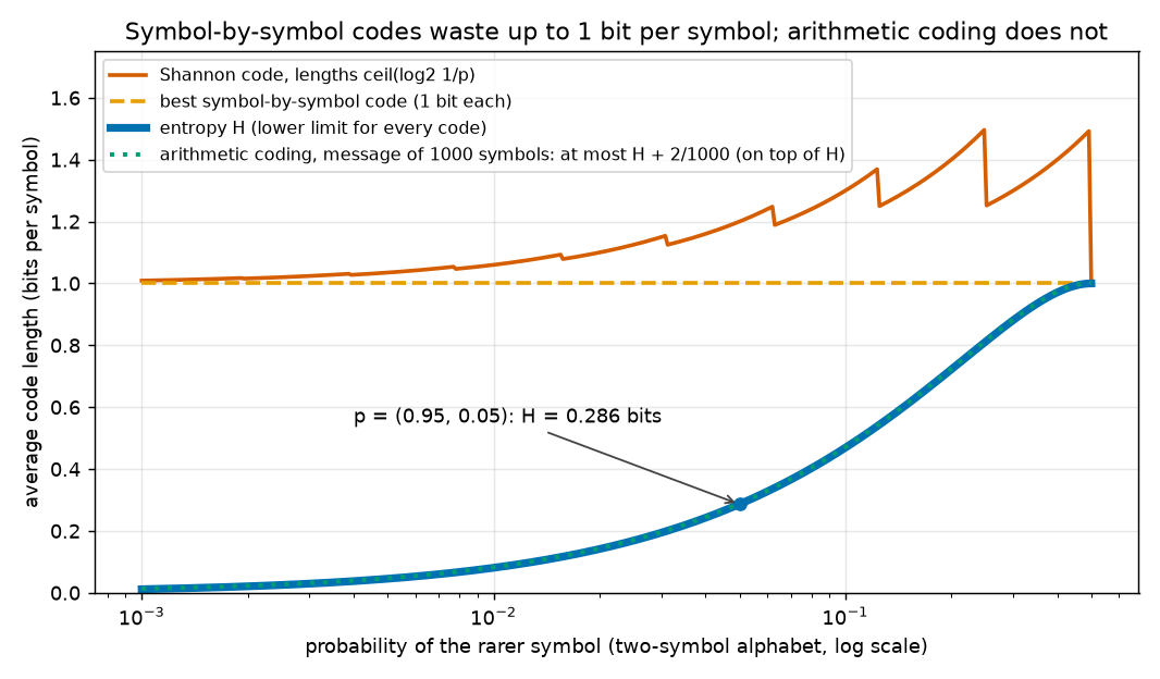
MY EXPLANATION With 11 or 17 quantization levels the waste is smaller, because no symbol of a moderately spread distribution is extremely likely. For our illustrative 11-level distribution below, the Huffman code (a standard symbol-by-symbol code built by repeatedly merging the two least likely symbols into one) costs 2.8478 bits per weight against an entropy of 2.8018. But on skewed weight distributions the waste can be large, and arithmetic coding removes it in all cases.

SOURCE: Lotfi et al. 2022, §4.2 The predecessor paper notes that for a small number of quantization levels, arithmetic coding compresses better than Huffman coding.

Arithmetic coding

Arithmetic coding is a code for whole messages. Fix the alphabet, the probabilities and the message length \(n\). Write \(F_k = p_1 + \cdots + p_{k-1}\) for the total probability of the symbols before \(k\) (so \(F_1 = 0\) and \(F_{L+1} = 1\)). Symbol \(k\) owns the piece \([F_k, F_{k+1})\) of the unit interval, of width \(p_k\).

Encoding (interval narrowing).

1. Start with the interval \([\text{low}, \text{low} + W) = [0, 1)\), so \(\text{low} = 0\) and the width is \(W = 1\).

2. For each symbol \(x_i\) of the message, in order, keep only the piece of the current interval that belongs to \(x_i\):

   \[ \text{low} \leftarrow \text{low} + W\cdot F_{x_i}, \qquad W \leftarrow W \cdot p_{x_i} . \]

3. After the last symbol, output the shortest bit string \(b = b_1 b_2\cdots b_k\) whose binary interval \([0.b_1 b_2\cdots b_k,\ 0.b_1 b_2 \cdots b_k + 2^{-k})\) lies entirely inside \([\text{low}, \text{low}+W)\). Here \(0.b_1 b_2\cdots b_k\) is the binary fraction \(b_1/2 + b_2/4 + \cdots + b_k/2^k\), and the binary interval contains exactly the numbers whose binary expansion starts with \(b\).

Decoding (the reverse process). The decoder knows the probabilities and \(n\). It reads \(v = 0.b_1\cdots b_k\) and repeats the zooming: at each step it splits the current interval into the pieces of the \(L\) symbols, finds the piece that contains \(v\), outputs that symbol, and keeps that piece. After \(n\) steps it stops.

The length theorem. The final width equals the probability of the message,

\[ W = p_{x_1} p_{x_2}\cdots p_{x_n}, \]

and the codeword has \(\lceil\log_2(1/W)\rceil\) or \(\lceil\log_2(1/W)\rceil + 1\) bits. Hence

\[ \text{length} \;\le\; \Big\lceil \log_2\frac{1}{W}\Big\rceil + 1 \;<\; \sum_{i=1}^{n}\log_2\frac{1}{p_{x_i}} + 2 \quad\text{bits}. \]

The sum on the right is the total surprisal of the message. For an i.i.d. source with distribution \(p\) its average is \(nH(p)\), so the expected length is below \(nH(p) + 2\) bits: within 2 bits of the source-coding bound for the whole message. For messages of a fixed length \(n\) the codewords form a prefix-free code.

Going deeper: proof that arithmetic coding works and costs at most 2 extra bits

MY EXPLANATION Setting. Alphabet \(\{1,\dots,L\}\), probabilities \(p_k > 0\) (a symbol with \(p_k = 0\) can be dropped from the alphabet), cumulative sums \(F_k\), a fixed message length \(n\). Write \(I(x_1\cdots x_i) = [\text{low}_i, \text{low}_i + W_i)\) for the interval after \(i\) symbols, with \(\text{low}_0 = 0\), \(W_0 = 1\). Nothing is random in the first five claims; they hold for every message.

Claim 1 (width = probability). \(W_i = p_{x_1}\cdots p_{x_i}\). By induction: \(W_0 = 1\) (the empty product), and each step multiplies the width by \(p_{x_i}\).

Claim 2 (the intervals tile). Fix a prefix \(x_1\cdots x_{i-1}\) with interval \([\ell, \ell + W)\). The \(L\) candidate next intervals are \([\ell + W F_k,\ \ell + W F_{k+1})\) for \(k = 1,\dots,L\). They are consecutive (each starts where the previous one ends), disjoint, and together they cover \([\ell + W F_1, \ell + W F_{L+1}) = [\ell, \ell + W)\). Consequence: if two messages of length \(n\) first differ at position \(i\), then after step \(i\) they sit in disjoint pieces of the same interval, and all their later intervals stay inside those pieces. So the \(L^n\) final intervals are disjoint (and together they cover \([0,1)\)).

Claim 3 (codeword length). Let \(W = W_n\), \(\ell = \text{low}_n\) and \(k_0 = \lceil\log_2(1/W)\rceil\), the smallest whole number with \(2^{-k_0} \le W\).

No shorter codeword is possible. A binary interval of width \(2^{-k}\) inside an interval of width \(W\) needs \(2^{-k} \le W\), so \(k \ge k_0\).

Length \(k_0 + 1\) always works. Let \(k = k_0 + 1\) and round \(\ell\) up to \(k\) binary digits: \(j = \lceil \ell\,2^k\rceil\). Then \(j\,2^{-k} \ge \ell\) and \(j\,2^{-k} < \ell + 2^{-k}\). The binary interval \([j2^{-k}, (j+1)2^{-k})\) therefore starts inside \([\ell, \ell + W)\) and ends before

\[ \ell + 2^{-k} + 2^{-k} = \ell + 2^{-k_0} \le \ell + W . \]

So the shortest codeword has \(k_0\) or \(k_0 + 1\) bits (the script tries exactly these two). With Claim 1,

\[ k \le \Big\lceil\log_2\frac{1}{\prod_i p_{x_i}}\Big\rceil + 1 < \log_2\frac{1}{\prod_i p_{x_i}} + 2 . \]

Claim 4 (prefix-free for a fixed length \(n\)). For a bit string \(b\) write \(J(b)\) for its binary interval. If \(b\) is a prefix of \(b'\) then \(J(b') \subseteq J(b)\) (Step 3 of the canonical-code proof in Chapter 12). Take two different messages \(x \ne x'\) with codewords \(b, b'\). Their binary intervals lie inside \(I(x)\) and \(I(x')\), which are disjoint (Claim 2). If \(b\) were a prefix of \(b'\), then \(J(b') \subseteq J(b) \subseteq I(x)\) and also \(J(b') \subseteq I(x')\), so the two disjoint intervals would share the non-empty set \(J(b')\). Contradiction. ∎

Claim 5 (decoding is correct). The number \(v = 0.b\) lies in \(J(b) \subseteq I(x_1\cdots x_n) \subseteq I(x_1\cdots x_i)\) for every \(i\), because the intervals are nested. Suppose the decoder has already recovered \(x_1,\dots,x_{i-1}\); then it knows \(I(x_1\cdots x_{i-1})\). By Claim 2 exactly one of the \(L\) pieces of that interval contains \(v\), and the piece of the true \(x_i\) does. So the decoder outputs \(x_i\). By induction it recovers the whole message. ∎

Why the decoder must know \(n\). Codes for different lengths are not prefix-free together. With \(p(a) = 1/2\), the one-letter message "a" has interval \([0, 1/2)\) and codeword 0, while "aa" has \([0, 1/4)\) and codeword 00. The string 00 could be "aa", or "a" followed by more bits. In the paper the number of symbols is \(d\), which the decoder learns from the hyperparameter bits (Chapter 24). Alternatives are an extra end-of-message symbol, or the length header of Chapter 12.

Claim 6 (expected length). Now let the message be random, from an i.i.d. source with distribution \(p\), and keep the coder fixed. Taking the expectation of Claim 3 and using \(\mathbb E\big[\log_2(1/\prod_i p_{X_i})\big] = \sum_i \mathbb E[\log_2(1/p_{X_i})] = nH(p)\) gives \(\mathbb E[\text{length}] < nH(p) + 2\) bits. With Shannon's lower bound applied to whole messages: \(nH(p) \le \mathbb E[\text{length}] < nH(p) + 2\).

A static model with empirical probabilities, and its header cost

PAPER App. E, p. 16; App. C, p. 15 The paper codes \(\hat w\) with the empirical probabilities: if level \(k\) occurs \(n_k\) times among the \(d\) weights, it uses \(\hat p_k = n_k/d\).

MY EXPLANATION A coder whose probabilities stay the same for every symbol is called a static model. With the empirical probabilities something neat happens: the total surprisal of the message is exactly \(d\) times the entropy of \(\hat p\),

\[ \log_2\frac{1}{\prod_{i=1}^{d}\hat p_{\hat w_i}} = \sum_{k=1}^{L_q} n_k\log_2\frac{1}{\hat p_k} = d\sum_{k=1}^{L_q}\hat p_k\log_2\frac{1}{\hat p_k} = d\,H(\hat p) , \]

because symbol \(k\) appears \(n_k = d\,\hat p_k\) times in the product. By the length theorem, the coded symbols take at most \(\lceil d\,H(\hat p)\rceil + 1 \le d\,H(\hat p) + 2\) bits.

There is a catch: the decoder needs the probabilities. The empirical probabilities are computed from \(\hat w\) itself, which depends on the training data. A decoder fixed before training cannot know them. So they must travel in the message, as a header in front of the coded symbols. The decoder also needs the codebook, the actual values of the levels, to turn symbols back into numbers.

SOURCE: Lotfi et al. 2022, §4.2 The predecessor paper counts \(d\,H(p) + 2\) bits for the coded weights, 16 bits per level for the codebook (half precision) and about \(\log_2 d\) bits per level for the probabilities, a total of about \(d\,H(p) + L_q(16 + \log_2 d) + 2\) bits.

[SOURCE: authors' code, sublora_bounds_quantize_fns.py] The public code adds 16 * len(codebook) bits for the codebook and ceil(log2(d)) * len(codebook) bits for the counts to the arithmetic-coded length. For \(d > 10{,}000\) it does not run the coder; it uses the formula \(\lceil d\,H(\hat p)\rceil + 1\) bits, which is the length the exact coder of this chapter is guaranteed to stay within (Claim 3 above).

MY EXPLANATION So the compressed size of the weights is

\[ C \approx \underbrace{\lceil d\,H(\hat p)\rceil + 1}_{\text{coded symbols}} + \underbrace{16\,L_q}_{\text{codebook}} + \underbrace{L_q\lceil\log_2 d\rceil}_{\text{counts}} \quad\text{bits}, \]

and then the paper adds the hyperparameter bits and the length header \(2\log_2 C\) of Chapter 12 (Algorithm 1 lines 19–20, whose bare "log" must be \(\log_2\) here, erratum E02).

Paper erratum E18: are the codebook and the counts counted?

PAPER App. C, Algorithm 1 lines 16–21, p. 15 GET_COMPRESSED_SIZE obtains the codebook values and the counts (line 17) and passes them to the arithmetic coder (line 18), but the pseudo-code never adds their size to message_size, and the text does not say whether they are counted.

MY EXPLANATION They must be, for the bound to be valid: without them the decoder cannot rebuild the intervals, and a code whose probabilities are chosen after seeing the trained weights is not a code fixed in advance (Chapter 12, last Going-deeper block). The authors' public code does count them, and their size is small: for \(d = 50{,}000\), 176 + 176 = 352 bits with 11 levels and 272 + 272 = 544 bits with 17 levels (script block [4]), against a message of about 140,000 bits. So the omission changes no reported number by more than a fraction of a percent of \(C(h)\).

Coding text with a language model

MY EXPLANATION Nothing in arithmetic coding requires the probabilities to stay the same. At step \(i\) the coder may split the interval according to any distribution, as long as the decoder can compute the same distribution. A language model provides exactly that: the probabilities \(p(x_i \mid x_{<i})\) of the next token given the tokens before it (Chapter 4). The decoder has the model and has already decoded \(x_{<i}\), so it can.

By the chain rule of probability, the final width is

\[ W = \prod_{i=1}^{n} p(x_i \mid x_{<i}) = p(x_1,\dots,x_n), \]

the probability of the whole text. By the length theorem the code takes fewer than

\[ \sum_{i=1}^{n}\log_2\frac{1}{p(x_i \mid x_{<i})} + 2 \quad\text{bits}, \]

which is the text's negative log-likelihood in bits (Chapter 6) plus at most 2. A better predictor is a better compressor, bit for bit. This is the sense in which "language modeling is compression".

SOURCE: Delétang et al. 2023 That phrase is the title of a paper the authors cite in §8 (p. 9), in a different context.

PAPER §7.1, p. 8–9; Fig. 3 right, p. 8 The paper forms a compression of the training set: the bits for the model, \(C(h)\), plus the bits for the data given the model, \(C(\{X\}_{i=1}^m \mid h)\), which it identifies with the negative log-likelihood of the whole dataset under the model. Figure 3 (right) plots the sum as "Compressed Dataset Size".

MY EXPLANATION This chapter supplies the missing step: arithmetic coding with the model achieves that NLL to within 2 bits per coded message, provided the NLL is measured in bits (\(\log_2\)). The decoder needs the model, which is why \(C(h)\) is added.

Paper erratum E59: the NLL that equals a code length must be in bits

PAPER §7.1, p. 8–9 The paper equates the number of bits needed to encode the data with "the negative log-likelihood of the entire dataset", without a log base.

MY EXPLANATION As a code length this holds only for the NLL in base 2, and only up to the coder's overhead (at most 2 bits per arithmetic-coded message). The paper's own Table 2 reports a "Validation NLL" in nats (erratum E27), so a reader who takes "NLL" in that sense would be off by a factor \(\ln 2 = 0.693\). The overhead is negligible: even if each of the \(m\) documents were coded as a separate message, it would add 16,019,524 bits, which is 0.0188 % of the plotted value (script block [7]). This adds to erratum E26 (the panel has no unit); no reported number changes.

Worked example with real numbers

Every number in this section is printed by ch22_arith_coder.py (output at the end of the chapter). Everything here is MY EXPLANATION unless tagged.

Step 1 — "abac" by hand

Alphabet \(\{a, b, c\}\) with \(p = (1/2, 1/4, 1/4)\), so \(a\) owns \([0, 1/2)\), \(b\) owns \([1/2, 3/4)\) and \(c\) owns \([3/4, 1)\) of the current interval.

After	Interval	Width	\(\log_2(1/\text{width})\)
(start)	\([0, 1)\)	1	0 bits
a	\([0, 1/2)\)	1/2	1 bit
ab	\([1/4, 3/8)\)	1/8	3 bits
aba	\([1/4, 5/16)\)	1/16	4 bits
abac	\([19/64, 5/16)\)	1/64	6 bits

Two of the steps in detail. After "a" the interval is \([0, 1/2)\) with \(W = 1/2\). The letter \(b\) has \(F_b = 1/2\) and \(p_b = 1/4\), so \(\text{low} = 0 + \tfrac12\cdot\tfrac12 = \tfrac14\) and \(W = \tfrac12\cdot\tfrac14 = \tfrac18\). At the last step \(c\) has \(F_c = 3/4\): \(\text{low} = \tfrac14 + \tfrac1{16}\cdot\tfrac34 = \tfrac{16}{64} + \tfrac{3}{64} = \tfrac{19}{64}\) and \(W = \tfrac1{16}\cdot\tfrac14 = \tfrac1{64}\).

The final width is \(\tfrac12\cdot\tfrac14\cdot\tfrac12\cdot\tfrac14 = \tfrac1{64}\), the probability of the message. The guaranteed length is at most \(\lceil\log_2 64\rceil + 1 = 7\) bits. Here 6 suffice: \(19/64\) in binary is \(0.010011\), and the binary interval of 010011 is \([19/64, 20/64)\), which is exactly the final interval (\(20/64 = 5/16\)). The codeword is 010011. The decoder, told \(n = 4\), reads \(v = 19/64\): it lies in \([0, 1/2)\), so the first letter is \(a\); and so on, giving back "abac".

The cost per letter is \(6/4 = 1.5\) bits, which is the entropy \(H(1/2, 1/4, 1/4) = 1.5000\) bits.

Step 2 — all messages of length 4 form a prefix-free code

The script encodes all \(3^4 = 81\) messages of length 4 and checks the claims of the length theorem:

Probabilities	Prefix-free?	Kraft sum	Mean length	\(4H\)	\(4H + 2\)
(1/2, 1/4, 1/4)	yes	1.0000	6.0000 bits	6.0000	8.0000
(3/5, 3/10, 1/10)	yes	0.5839	6.0500 bits	5.1818	7.1818

With probabilities that are powers of 1/2 every interval is itself a binary interval, so there is no waste at all: the mean length equals the entropy bound. With (0.6, 0.3, 0.1) the code pays 0.8682 bits above \(4H\) for the whole message, within the promised 2 bits. Every message decodes correctly.

Step 3 — entropy against symbol-by-symbol codes

Distribution	\(H\) (bits)	Shannon code	Huffman code	Fixed length
(1/2, 1/4, 1/4)	1.5000	1.5000	1.5000	2
(0.6, 0.3, 0.1)	1.2955	1.6000	1.4000	2
(0.95, 0.05)	0.2864	1.2000	1.0000	1
11 levels, Step 5	2.8018	3.5881	2.8478	4

All columns are in bits per symbol. Every code is at least \(H\), as the source-coding bound demands, and the Shannon code is below \(H + 1\).

Step 4 — the exact coder on 2,000 quantized weights

The script draws 2,000 numbers from a standard normal distribution (seed 1) and rounds each to the nearest of 11 equally spaced levels, 0.6 standard deviations apart. This imitates the shape of a quantized weight vector: most weights near the middle levels. It is an illustration, not the paper's data. The level counts are 10, 30, 89, 256, 401, 473, 399, 210, 93, 31, 8.

• Entropy of the empirical frequencies: \(H(\hat p) = 2.8015\) bits per symbol, so \(d\,H(\hat p) = 5603.07\) bits.
• The exact final width, computed with fractions, gives \(\log_2(1/W) = 5603.07\) bits: equal to \(d\,H(\hat p)\), as the identity above says.
• The codeword has 5,604 bits, within the guarantee \(\lceil dH\rceil + 1 = 5{,}605\) bits. It decodes back exactly.
• A 32-bit integer coder (the finite-precision kind used in practice) produces 5,604 bits too.
• A fixed 4-bit code would take 8,000 bits.

Step 5 — the full bit budget for d = 50,000 weights

Same recipe, now with \(d = 50{,}000\) weights (seed 0). The level counts are 178, 740, 2,395, 5,892, 9,875, 11,717, 9,973, 5,903, 2,435, 715, 177, and \(H(\hat p) = 2.8018\) bits per weight (the maximum for 11 levels is 3.4594).

Item	Bits
Fixed length, 4 bits per weight (for comparison)	200,000 (24.414 KB)
Ideal for uniform levels, \(d\log_2 11\) (for comparison)	172,971.6
\(d\,H(\hat p)\)	140,088.1
Coded symbols, exact coder, \(\lceil dH\rceil + 1\)	140,090
Coded symbols, 32-bit integer coder (actually run)	140,089
Codebook, 16 bits × 11 levels	176
Counts, 11 × \(\lceil\log_2 50{,}000\rceil\) = 11 × 16	176
Message \(C\)	140,442
Length header, \(2\log_2 C\) (Elias gamma: 35)	34.2
Total	140,476.2 = 17.148 KB

The total is 2.8095 bits per weight. A fixed-length code with its codebook and header would take 200,211.2 bits (24.440 KB), so arithmetic coding saves 29.8 %. The header for codebook and counts is 352 bits, 0.25 % of the total. The hyperparameter bits of Algorithm 1 line 19 come on top (Chapter 24).

With 17 levels the codebook and the counts would take 272 + 272 = 544 bits, and a fixed-length code 5 bits per weight, 250,000 bits.

Step 6 — what the paper's compressed sizes imply

[PAPER Fig. 2 left, p. 5; read exactly by fig_extract.py] Figure 2 (left) plots the compressed size against the subspace dimension \(d\). Dividing by \(d\) (with 1 KB = 8,192 bits, erratum E35):

\(d\)	5,000	7,500	10,000	25,000	50,000	75,000	100,000	200,000
Size (KB)	2.1124	2.5564	3.8782	9.8081	16.5325	27.9915	35.7461	57.3441
Bits per weight	3.461	2.792	3.177	3.214	2.709	3.057	2.928	2.349

MY EXPLANATION Every point spends between 2.349 and 3.461 bits per weight, everything included that the paper counts. That is well below the 4 or 5 bits of a fixed-length code for 11 or 17 levels, and below \(\log_2 11 = 3.4594\) except at \(d = 5{,}000\), where headers of a few hundred bits are spread over only 5,000 weights. The best model, \(d = 50{,}000\) at 135,434 bits, spends 2.709 bits per weight, close to the 2.8 bits of our illustrative distribution. We cannot split these totals into entropy and headers: the paper reports neither the number of levels of each point nor the level counts (errata E18, E33). (Fig. 2 also has points at \(d\) = 7,500 and 75,000, which are not in the App. E grid; see erratum E40.)

Step 7 — a language model as a compressor

The script trains a character bigram model (Chapter 4) on a 537-character paragraph, with add-one smoothing so that no character gets probability 0. (A zero probability would make the interval width 0 and the code length infinite; Chapter 16 meets the same problem for LLMs.) The alphabet has 29 symbols: 26 letters, space, period and comma. It then codes a different 94-character sentence.

Way to store the sentence	Bits	Bits per character
8 bits per character	752	8
Uniform over 29 symbols, \(94\log_2 29\)	456.65	4.858
NLL of the sentence under the bigram model	325.80	3.466
Arithmetic code with the bigram model (actually run)	327	—

The arithmetic code is 1.2 bits above the NLL, within the promised 2, and decodes back exactly.

[PAPER Fig. 3 right, p. 8; read by fig_extract.py] At the largest model of Figure 3, the "Compressed Dataset Size" is \(8.5028\times10^{10}\) (bits, presumably; erratum E26).

[SOURCE: nanoGPT prepare.py] The OpenWebText training split has 9,035,582,198 tokens and 8,009,762 documents.

MY EXPLANATION So the plotted size corresponds to 9.410 bits per training token (9.391–9.910 along the plotted best-bound line). The model's own bits are negligible: a 20 KB model is 163,840 bits, \(1.93\times10^{-6}\) of the total. The panel is essentially the training NLL in bits. Chapter 26 discusses what it does and does not show.

Going deeper

Everything in this section is MY EXPLANATION unless tagged.

The proofs sit next to the definitions they support:

• "Proof of Gibbs' inequality" and "Entropy lies between 0 and log2 L" — under Entropy and Gibbs' inequality.
• "Proof of the source-coding bound" and "The Shannon code reaches H + 1" — under Shannon's source-coding bound.
• "Proof that arithmetic coding works and costs at most 2 extra bits" — under Arithmetic coding.

Three more blocks follow here.

Going deeper: the cheapest way to pay for the probabilities

MY EXPLANATION Why a two-part code is a legal code. The scheme "first the counts \(n_1,\dots,n_{L_q}\) in fixed-length binary, then the codebook, then the arithmetic code of \(\hat w\) built from \(\hat p_k = n_k/d\)" is one rule fixed before training. The data only decide which codeword is used. Each part is prefix-free once the earlier parts are known: the counts and codebook have fixed lengths, and the arithmetic part is prefix-free for the known length \(d\) (Claim 4). By the joining lemma of Chapter 12 the whole description is prefix-free, so its length can serve as \(C(h)\).

Counts in \(\lceil\log_2 d\rceil\) bits. A count lies between 0 and \(d\), which is \(d + 1\) possible values, so in general \(\lceil\log_2(d+1)\rceil\) bits are needed. The two differ only when \(d\) is a power of 2. For \(d = 50{,}000\), 16 bits suffice because \(2^{16} = 65{,}536 > 50{,}000\); none of the paper's \(d\) values is a power of 2. Also, the last count is redundant, since all counts add up to \(d\).

The number of messages with given counts. How many sequences of length \(d\) have exactly the counts \(n_k\)? The multinomial coefficient \(d!/(n_1!\cdots n_{L_q}!)\). It is at most \(2^{d H(\hat p)}\). Proof: by the multinomial theorem,

\[ 1 = \Big(\sum_k \hat p_k\Big)^{d} = \sum_{m_1+\dots+m_{L_q} = d}\frac{d!}{\prod_k m_k!}\prod_k \hat p_k^{\,m_k} \;\ge\; \frac{d!}{\prod_k n_k!}\prod_k \hat p_k^{\,n_k} = \frac{d!}{\prod_k n_k!}\,2^{-d H(\hat p)} , \]

keeping only the term \(m = n\) (all terms are \(\ge 0\)), and using \(\prod_k \hat p_k^{n_k} = 2^{-dH(\hat p)}\) (the identity for empirical probabilities above). For Step 5: \(\log_2(d!/\prod_k n_k!) = 140{,}021.9\) bits, just below \(d\,H(\hat p) = 140{,}088.1\).

The number of possible count vectors. Lists of \(L_q\) counts that add up to \(d\) correspond to arrangements of \(d\) "stars" and \(L_q - 1\) "bars", so there are \(\binom{d + L_q - 1}{L_q - 1}\) of them. Naming one costs \(\log_2\binom{d+L_q-1}{L_q-1}\) bits: 134.3 bits for \(d = 50{,}000\), \(L_q = 11\), instead of the 176 bits of fixed-length counts.

An adaptive coder needs no header at all. The Laplace adaptive coder codes symbol \(t+1\) with probabilities \((m_k + 1)/(t + L_q)\), where \(m_k\) counts how often level \(k\) appeared among the first \(t\) symbols. The decoder can keep the same counts as it decodes, so nothing needs to be sent in advance. The probability it gives the whole message is a product whose numerators, for level \(k\), are \(1, 2, \dots, n_k\) (one per occurrence) and whose denominators are \(L_q, L_q + 1, \dots, L_q + d - 1\). So

\[ \log_2\frac{1}{W} = \log_2\frac{(d + L_q - 1)!}{(L_q - 1)!\,\prod_k n_k!} = \log_2\binom{d+L_q-1}{L_q-1} + \log_2\frac{d!}{\prod_k n_k!} , \]

exactly "name the count vector" plus "name the sequence among those with these counts". For Step 5 this is 140,156.2 bits, against \(d\,H(\hat p) + 352 = 140{,}440.1\) bits for the static code with its header. The saving, about 284 bits, is 0.2 % of the message. The paper's simpler choice costs almost nothing.

Going deeper: arithmetic coding with 32-bit integers (what real coders do)

MY EXPLANATION The algorithm (the design of Witten, Neal and Cleary, 1987, used by the script). Keep an integer range \([\text{low}, \text{high}]\) inside \([0, 2^{32} - 1]\) and integer cumulative counts \(c_k = n_1 + \dots + n_{k-1}\) with total \(T = d\). To code symbol \(k\), with \(R = \text{high} - \text{low} + 1\):

\[ \text{high} \leftarrow \text{low} + \lfloor R\,c_{k+1}/T\rfloor - 1, \qquad \text{low} \leftarrow \text{low} + \lfloor R\,c_k/T\rfloor . \]

Then renormalize: while the range lies in the lower half, output 0; while it lies in the upper half, output 1 and subtract half; while it straddles the midpoint inside the middle half, remember one "pending" bit (its value is decided later) and subtract a quarter; after each of these, double low and high (high becomes \(2\,\text{high}+1\)). At the end, output two more bits that pin a quarter of the integer range lying inside the final range.

Range after renormalization. The loop stops only when \(\text{low} < 2^{31} \le \text{high}\) and not both \(\text{low} \ge 2^{30}\) and \(\text{high} < 3\cdot 2^{30}\). Either \(\text{low} < 2^{30}\) (then \(R > 2^{31} - 2^{30} = 2^{30}\)) or \(\text{high} \ge 3\cdot2^{30}\) (then \(R > 3\cdot 2^{30} - 2^{31} = 2^{30}\)). So every symbol is coded with \(R > 2^{30}\).

Length bound. Each pass of the loop doubles \(R\) exactly (\(2\,\text{high} + 1 - 2\,\text{low} + 1 = 2R\)) and produces exactly one output bit, now or later. Subtracting a half or a quarter does not change \(R\). Coding symbol \(x_i\) multiplies \(R\) by \(r_i = \big(\lfloor R c_{k+1}/T\rfloor - \lfloor R c_k/T\rfloor\big)/R\). If the loop runs \(N\) times in total, the final range is \(2^{32}\big(\prod_i r_i\big)2^{N} \le 2^{32}\), so \(N \le \log_2(1/\prod_i r_i)\). The output has \(N + 2\) bits.

Since \(\lfloor a\rfloor > a - 1\) and \(\lfloor b\rfloor \le b\), the new range exceeds \(R\,n_k/T - 1\), so

\[ r_i > \hat p_k - \frac1R \ge \hat p_k\Big(1 - \frac{T}{R\,n_k}\Big) \ge \hat p_k\Big(1 - \frac{T}{2^{30}}\Big), \]

using \(n_k \ge 1\) and \(R > 2^{30}\). (This also shows that no symbol ever gets an empty range, as long as \(T \le 2^{30}\).) Taking \(\log_2\) and adding over the \(d\) symbols:

\[ \text{length} = N + 2 < d\,H(\hat p) + 2 + d\log_2\frac{1}{1 - T/2^{30}} . \]

For \(d = T = 50{,}000\) the last term is 3.36 bits for the whole message. The script's integer coder used 140,089 bits, one bit less than the exact coder's guarantee, because the rounding favours some symbols and penalises others.

Decoding. The decoder mirrors the encoder: it keeps the same integer range plus a 32-bit window of the code bits, and at each step finds the symbol whose integer sub-range contains the window. We skip the proof that it always picks the right symbol (it is the integer version of Claim 5, with care at the rounding boundaries); the script checks the round trip on all 50,000 symbols.

Going deeper: coding with a language model, and why NLL is a code length

MY EXPLANATION Setting. A model gives, for every position \(i\) and every possible earlier text \(x_{<i}\), a distribution \(q(\cdot \mid x_{<i})\) over the next token with all probabilities positive (prediction smoothing, Chapter 16, guarantees this). The encoder and the decoder both have the model.

The coder. At step \(i\), split the current interval in proportion to \(q(\cdot \mid x_{<i})\). Claims 1–5 of the arithmetic-coding proof go through word for word, with \(p_{x_i}\) replaced by \(q(x_i \mid x_{<i})\): the decoder knows \(x_{<i}\) when it needs the distribution. By the chain rule the final width is \(q(x_1,\dots,x_n)\), and the length is below \(\log_2\frac{1}{q(x_1,\dots,x_n)} + 2\) bits.

Average over texts. If texts are drawn from a true distribution \(p\) (random) and the model \(q\) is fixed, the expected length is below \(\mathbb E_p\big[\log_2\frac{1}{q(X)}\big] + 2\), the cross-entropy plus 2. By Gibbs this is at least the entropy of the text distribution, the floor for every code. The gap is the KL divergence between the true distribution and the model: every bit by which a model's average NLL exceeds the floor is a bit of compression lost.

Per document or per corpus. Coding each of \(m\) documents separately costs at most \(2m\) extra bits; coding the whole corpus as one message costs at most 2. The decoder must also learn where documents end; GPT-2's vocabulary has an end-of-text token for this (Chapter 4), whose probability is then part of the NLL.

Common misconceptions

• Misconception: "Entropy is a property of a single message." — Actually: it is a property of a distribution: the average surprisal. The code length of one particular message is its own surprisal, \(\sum_i\log_2(1/p_{x_i})\), which can be above or below \(nH(p)\); with empirical probabilities the two coincide exactly.
• Misconception: "A clever enough code can beat the entropy on average." — Actually: no uniquely decodable code can (source-coding bound, proved by Kraft/McMillan plus Gibbs). Arithmetic coding gets within 2 bits of it for a whole message, which is per-symbol perfection for long messages.
• Misconception: "Arithmetic coding sends one fraction per symbol." — Actually: it sends one binary fraction for the whole message. That is why it avoids the up-to-1-bit-per-symbol waste of symbol-by-symbol codes (0.7136 bits per symbol for probabilities 0.95 and 0.05).
• Misconception: "The compressed size is just \(d\,H(\hat p)\)." — Actually: the decoder also needs the codebook, the counts (or another way to get the probabilities), the number of symbols and a length header. For \(d = 50{,}000\) and 11 levels the codebook and counts add 352 bits and the length header 34.2 bits to the 140,090 bits of coded symbols: small, but required for a valid bound (erratum E18).
• Misconception: "Using probabilities computed from the weights themselves is cheating." — Actually: it is legal as long as the probabilities (the counts) are sent in the message. The rule "send counts, then code with them" is fixed in advance; only its output depends on the data.
• Misconception: "An exact arithmetic coder needs infinite precision, so the formula \(\lceil dH\rceil + 1\) is only a theoretical number." — Actually: a 32-bit integer coder reaches it within a guaranteed 3.36 bits for \(d = 50{,}000\), and in the script it even matched it.

Self-test

Q1. (numeric) With \(p(a) = 1/2\), \(p(b) = 1/4\), \(p(c) = 1/4\), encode the message "cab". Give the final interval, its width, and the shortest codeword.

Answer

\(c\) owns \([3/4, 1)\), so after "c" the interval is \([3/4, 1)\), width 1/4. Then \(a\) takes the first half: \([3/4, 7/8)\), width 1/8. Then \(b\) takes the piece from \(F_b = 1/2\) to \(3/4\) of the current interval: \(\text{low} = 3/4 + \tfrac18\cdot\tfrac12 = 13/16\), width \(\tfrac18\cdot\tfrac14 = 1/32\). The final interval is \([13/16, 27/32)\) of width \(1/32 = 2^{-5}\), so at least 5 bits are needed. \(13/16 = 26/32\) is \(0.11010\) in binary, and the binary interval of 11010 is \([26/32, 27/32)\), exactly the final interval. Codeword: 11010 (5 bits). This equals the total surprisal, \(\log_2 4 + \log_2 2 + \log_2 4 = 2 + 1 + 2 = 5\) bits. The script prints the same (block [1]).

Q2. (conceptual) A colleague computes \(C(h)\) as \(\lceil d\,H(\hat p)\rceil + 1\) and stops there. What is missing, and why does it matter for the validity of the bound, not only for its tightness?

Answer

The decoder cannot rebuild the intervals without the probabilities \(\hat p_k\) (sent as counts), cannot turn symbols into weights without the codebook, and needs to know \(d\) (paid in the hyperparameter bits) and the total message length (the length header). The probabilities are computed from the trained weights, so they depend on the training data. Leaving them out means the "code" was chosen after seeing the data, which breaks the requirement that the prior, hence the code, be fixed in advance (Chapter 12). Adding them back costs only a few hundred bits (352 for \(d = 50{,}000\), \(L_q = 11\)), so the fix is cheap, but without it the stated guarantee does not follow. This is erratum E18.

Q3. (numeric) For \(d = 50{,}000\) weights on 17 levels instead of 11, how many bits do the codebook and the counts take, and how many bits would a fixed-length code need for the symbols? Compare with the 11-level numbers of Step 5.

Answer

Codebook: \(16 \times 17 = 272\) bits. Counts: \(17\times\lceil\log_2 50{,}000\rceil = 17 \times 16 = 272\) bits. Together 544 bits (script block [4]), against 352 bits with 11 levels. A fixed-length code needs \(\lceil\log_2 17\rceil = 5\) bits per weight, \(5 \times 50{,}000 = 250{,}000\) bits, against 200,000 bits with 11 levels. With arithmetic coding the symbols cost about \(d\,H(\hat p)\) bits whatever the number of levels, and \(H(\hat p) \le \log_2 17 = 4.0875\); more levels only pay if the better-fitting weights lower the training loss by more than the extra entropy and header cost. The header stays a fraction of a percent of the message either way.

Code for this chapter

Run it from the project root:

.venv/Scripts/python explainer/code/ch22_arith_coder.py

Source: ch22_arith_coder.py

"""Chapter 22 demo: entropy, symbol codes and a tiny exact arithmetic coder.

What this script reproduces or illustrates (every number quoted in Chapter 22 comes from here):
  [1] Interval narrowing for the message "abac" with p(a)=1/2, p(b)=1/4, p(c)=1/4, in exact fractions
      (Python fractions.Fraction); the final width is the product of the symbol probabilities (1/64);
      the shortest codeword whose binary interval fits inside; decoding back. All 81 messages of length 4
      for two distributions: the codewords form a prefix-free code; Kraft sum; mean length vs 4 H(p).
  [2] Entropy H(p) versus symbol-by-symbol codes (Shannon code, Huffman code, fixed length) - the up-to-
      1-bit-per-symbol waste of symbol codes on skewed distributions.
  [3] The exact coder on a random 2,000-symbol sequence over L_q = 11 levels with its EMPIRICAL
      probabilities: -log2(final width) = d H(p_hat) exactly; length <= ceil(d H)+1 <= d H + 2; round trip.
      Same sequence with a 32-bit integer coder (Witten-Neal-Cleary style, finite precision).
  [4] Bit accounting for d = 50,000 quantized weights over L_q = 11 levels (illustrative discretized
      Gaussian, seed 0), following Lotfi et al. (2022, Sec. 4.2): d H + 2 bits for the symbols, 16 L_q bits
      for a half-precision codebook, L_q ceil(log2 d) bits for the counts (erratum E18); the length header
      of Chapter 12; integer coder actually run on all 50,000 symbols; cheaper ways to pay for the counts.
  [5] [PAPER Fig. 2 left] compressed sizes (read exactly by fig_extract.py) -> bits per subspace weight.
  [6] Coding text with a language model (character bigram, add-one smoothing): code length vs the
      text's negative log-likelihood in bits ("language modeling is compression").
  [7] [PAPER Fig. 3 right] "compressed dataset size" per training token (fig_extract.py data).
Figures: docs/assets/fig/ch22_intervals.png, docs/assets/fig/ch22_waste.png
Output:  code/outputs/ch22_arith_coder.txt
Deterministic (numpy default_rng seeds 0 and 1). Runtime: a few seconds on a laptop CPU.
"""
from __future__ import annotations

import heapq
import itertools
import json
import math
import sys
import time
from fractions import Fraction
from pathlib import Path

import numpy as np
import matplotlib

matplotlib.use("Agg")
import matplotlib.pyplot as plt  # noqa: E402

HERE = Path(__file__).resolve().parent
sys.path.insert(0, str(HERE))
import pacbound as pb  # noqa: E402

OUT_TXT = HERE / "outputs" / "ch22_arith_coder.txt"
FIG_DIR = HERE.parent / "docs" / "assets" / "fig"
FIG_INT = FIG_DIR / "ch22_intervals.png"
FIG_WASTE = FIG_DIR / "ch22_waste.png"
FIG_JSON = HERE / "outputs" / "fig_extract.json"
OUT_TXT.parent.mkdir(parents=True, exist_ok=True)
FIG_DIR.mkdir(parents=True, exist_ok=True)

LINES: list[str] = []


def say(s: str = "") -> None:
    print(s)
    LINES.append(s)


# ---------------------------------------------------------------------------
# Entropy and symbol codes
# ---------------------------------------------------------------------------
def entropy_bits(p) -> float:
    """H(p) = -sum p_k log2 p_k in bits per symbol (terms with p_k = 0 contribute 0)."""
    return -sum(float(x) * math.log2(float(x)) for x in p if x > 0)


def shannon_lengths(p) -> list[int]:
    """Shannon code lengths ceil(-log2 p_k) (exact for Fractions that are powers of 1/2)."""
    out = []
    for x in p:
        x = Fraction(x)
        k = 0
        while Fraction(1, 2 ** k) > x:      # smallest k with 2^-k <= p_k
            k += 1
        out.append(k)
    return out


def huffman_lengths(p) -> list[int]:
    """Codeword lengths of a Huffman code (repeatedly merge the two least likely groups)."""
    if len(p) == 1:
        return [1]
    heap = [(float(x), i, [i]) for i, x in enumerate(p)]
    heapq.heapify(heap)
    lengths = [0] * len(p)
    tie = len(p)
    while len(heap) > 1:
        a = heapq.heappop(heap)
        b = heapq.heappop(heap)
        for i in a[2] + b[2]:
            lengths[i] += 1
        heapq.heappush(heap, (a[0] + b[0], tie, a[2] + b[2]))
        tie += 1
    return lengths


def mean_length(p, lengths) -> float:
    return sum(float(x) * l for x, l in zip(p, lengths))


# ---------------------------------------------------------------------------
# Exact arithmetic coder (fractions.Fraction); "model" maps the previous symbol to (probs, cum)
# ---------------------------------------------------------------------------
def with_cum(probs):
    probs = [Fraction(x) for x in probs]
    assert sum(probs) == 1 and all(x > 0 for x in probs)
    cum = [Fraction(0)]
    for x in probs:
        cum.append(cum[-1] + x)
    return probs, cum


def ceil_neg_log2(width: Fraction) -> int:
    """Exact ceil(-log2 width) for 0 < width <= 1: the smallest k >= 0 with 2^k * width >= 1."""
    k = max(0, (width.denominator // width.numerator).bit_length() - 1)
    while width * (1 << k) < 1:
        k += 1
    while k > 0 and width * (1 << (k - 1)) >= 1:
        k -= 1
    return k


def shortest_codeword(low: Fraction, high: Fraction) -> str:
    """Shortest bit string b = b1..bk whose binary interval [0.b, 0.b + 2^-k) lies inside [low, high).
    Only k0 = ceil(-log2(high-low)) and k0 + 1 can be the answer (proved in the chapter)."""
    k0 = ceil_neg_log2(high - low)
    for k in (k0, k0 + 1):
        j = math.ceil(low * (1 << k))          # round low UP to k binary digits
        if Fraction(j + 1, 1 << k) <= high:
            return format(j, f"0{k}b") if k > 0 else ""
    raise AssertionError("unreachable: k0 + 1 always works")


def ac_encode(seq, model, trace=False):
    """Interval narrowing. model(prev) -> (probs, cum); prev is None for the first symbol."""
    low, width = Fraction(0), Fraction(1)
    steps = [(low, width)]
    prev = None
    for s in seq:
        probs, cum = model(prev)
        low += width * cum[s]
        width *= probs[s]
        prev = s
        if trace:
            steps.append((low, width))
    return shortest_codeword(low, low + width), low, width, steps


def ac_decode(bits: str, n: int, model):
    """Reverse process: needs the bits, the number of symbols n and the same model."""
    v = Fraction(int(bits, 2), 1 << len(bits)) if bits else Fraction(0)
    low, width = Fraction(0), Fraction(1)
    out, prev = [], None
    for _ in range(n):
        probs, cum = model(prev)
        s = 0
        while v >= low + width * cum[s + 1]:   # find the sub-interval that contains v
            s += 1
        low += width * cum[s]
        width *= probs[s]
        out.append(s)
        prev = s
    return out


def static(probs):
    pc = with_cum(probs)
    return lambda prev: pc


# ---------------------------------------------------------------------------
# Finite-precision integer arithmetic coder (32-bit, Witten-Neal-Cleary 1987 style)
# ---------------------------------------------------------------------------
PREC = 32
TOP, HALF, QTR = (1 << PREC) - 1, 1 << (PREC - 1), 1 << (PREC - 2)


def int_encode(seq, counts):
    cumf = [0] + list(itertools.accumulate(counts))
    T = cumf[-1]
    assert T <= QTR
    low, high, pending, out = 0, TOP, 0, []

    def emit(bit):
        nonlocal pending
        out.append(bit)
        out.extend([1 - bit] * pending)
        pending = 0

    for s in seq:
        rng = high - low + 1
        high = low + rng * cumf[s + 1] // T - 1
        low = low + rng * cumf[s] // T
        while True:
            if high < HALF:
                emit(0)
            elif low >= HALF:
                emit(1)
                low -= HALF
                high -= HALF
            elif low >= QTR and high < 3 * QTR:
                pending += 1
                low -= QTR
                high -= QTR
            else:
                break
            low, high = 2 * low, 2 * high + 1
    pending += 1                       # termination: two more bits pin a quarter inside [low, high]
    emit(0 if low < QTR else 1)
    return out


def int_decode(bits, n, counts):
    cumf = [0] + list(itertools.accumulate(counts))
    T = cumf[-1]
    it = iter(bits)
    nxt = lambda: next(it, 0)          # pad with zeros after the end of the message
    value = 0
    for _ in range(PREC):
        value = 2 * value + nxt()
    low, high, out = 0, TOP, []
    for _ in range(n):
        rng = high - low + 1
        target = ((value - low + 1) * T - 1) // rng
        s = 0
        while cumf[s + 1] <= target:
            s += 1
        out.append(s)
        high = low + rng * cumf[s + 1] // T - 1
        low = low + rng * cumf[s] // T
        while True:
            if high < HALF:
                pass
            elif low >= HALF:
                value -= HALF
                low -= HALF
                high -= HALF
            elif low >= QTR and high < 3 * QTR:
                value -= QTR
                low -= QTR
                high -= QTR
            else:
                break
            low, high = 2 * low, 2 * high + 1
            value = 2 * value + nxt()
    return out


# ---------------------------------------------------------------------------
# Quantized "weights": 11 equally spaced levels, spacing 0.6 standard deviations (illustrative)
# ---------------------------------------------------------------------------
LQ = 11
SPACING = 0.6


def quantize(x):
    """Nearest of the levels (k - 5) * SPACING, k = 0..10 (x in units of its standard deviation)."""
    return np.clip(np.rint(x / SPACING).astype(int) + 5, 0, LQ - 1)


def main() -> None:
    t_start = time.time()
    # =======================================================================
    say("[1] Interval narrowing for 'abac', p(a)=1/2, p(b)=1/4, p(c)=1/4 (exact fractions)")
    P3 = [Fraction(1, 2), Fraction(1, 4), Fraction(1, 4)]
    names = "abc"
    msg = [names.index(ch) for ch in "abac"]
    code, low, width, steps = ac_encode(msg, static(P3), trace=True)
    labels = ["start", "after a", "after ab", "after aba", "after abac"]
    for lab, (lo, w) in zip(labels, steps):
        say(f"  {lab:<11} [{str(lo):>5}, {str(lo + w):>5})  width {str(w):>4}"
            f"  -log2(width) = {abs(math.log2(w)):.0f} bits")
    prod = Fraction(1, 2) * Fraction(1, 4) * Fraction(1, 2) * Fraction(1, 4)
    assert width == prod == Fraction(1, 64)
    dec = "".join(names[s] for s in ac_decode(code, 4, static(P3)))
    assert dec == "abac" and code == "010011"
    say(f"  codeword {code} ({len(code)} bits): binary interval [{Fraction(int(code, 2), 64)}, "
        f"{Fraction(int(code, 2) + 1, 64)}); guaranteed <= ceil(-log2 W)+1 = {ceil_neg_log2(width) + 1}")
    say(f"  decoded back with n = 4 symbols: '{dec}'")
    c_cab, lo_cab, w_cab, _ = ac_encode([2, 0, 1], static(P3))
    assert ac_decode(c_cab, 3, static(P3)) == [2, 0, 1]
    say(f"  self-test 'cab': final [{lo_cab}, {lo_cab + w_cab}), width {w_cab}, codeword {c_cab}"
        f" ({len(c_cab)} bits)")
    for P in (P3, [Fraction(3, 5), Fraction(3, 10), Fraction(1, 10)]):
        words, mean, kraft = [], 0.0, Fraction(0)
        for seq in itertools.product(range(3), repeat=4):
            c, _, w, _ = ac_encode(seq, static(P))
            assert ac_decode(c, 4, static(P)) == list(seq)
            assert len(c) <= ceil_neg_log2(w) + 1
            words.append(c)
            mean += float(w) * len(c)          # w = probability of the message
            kraft += Fraction(1, 2 ** len(c))
        sw = sorted(words)
        pf = len(set(words)) == len(words) and not any(b.startswith(a) for a, b in zip(sw, sw[1:]))
        H = entropy_bits(P)
        say(f"  all 81 messages of length 4, p = ({', '.join(str(x) for x in P)}): "
            f"prefix-free = {pf}, Kraft sum = {float(kraft):.4f}")
        say(f"      mean codeword length {mean:.4f} bits; 4H = {4 * H:.4f}, 4H + 2 = {4 * H + 2:.4f} bits;"
            f" excess {mean - 4 * H:.4f}")
        assert pf and kraft <= 1 and 4 * H <= mean <= 4 * H + 2

    # =======================================================================
    rng0 = np.random.default_rng(0)
    d = 50_000
    sym50 = quantize(rng0.standard_normal(d))
    n50 = np.bincount(sym50, minlength=LQ)
    p50 = [Fraction(int(c), d) for c in n50]
    H50 = entropy_bits(p50)

    say("[2] Entropy vs symbol-by-symbol codes (bits per symbol)")
    say("  distribution                       H      Shannon  Huffman  fixed")
    rows = [("(1/2, 1/4, 1/4)", P3), ("(0.6, 0.3, 0.1)", [Fraction(3, 5), Fraction(3, 10), Fraction(1, 10)]),
            ("(0.95, 0.05)", [Fraction(19, 20), Fraction(1, 20)]),
            ("11 levels, d=50,000 (sec. [4])", p50)]
    for name, P in rows:
        sl, hl = shannon_lengths(P), huffman_lengths(P)
        assert sum(Fraction(1, 2 ** l) for l in sl) <= 1          # Shannon lengths satisfy Kraft
        H, ms, mh = entropy_bits(P), mean_length(P, sl), mean_length(P, hl)
        assert H <= mh <= ms < H + 1
        say(f"  {name:<32} {H:6.4f}  {ms:6.4f}   {mh:6.4f}   {math.ceil(math.log2(len(P)))}")
    say(f"  (0.95, 0.05): best symbol code wastes 1 - H = {1 - entropy_bits([0.95, 0.05]):.4f} bits/symbol;"
        f" log2(1/0.95) = {math.log2(1 / 0.95):.4f} bits")
    say(f"  log2 11 = {math.log2(11):.4f}, log2 17 = {math.log2(17):.4f} bits (fixed length: 4 and 5 bits)")

    # =======================================================================
    say("[3] Exact coder on 2,000 symbols over 11 levels, empirical probabilities (seed 1)")
    rng1 = np.random.default_rng(1)
    n2 = 2000
    seq2 = [int(s) for s in quantize(rng1.standard_normal(n2))]
    cnt2 = np.bincount(seq2, minlength=LQ)
    used = [k for k in range(LQ) if cnt2[k] > 0]          # an empty bin gets probability 0: drop it
    remap = {k: i for i, k in enumerate(used)}
    p2 = [Fraction(int(cnt2[k]), n2) for k in used]
    s2 = [remap[s] for s in seq2]
    t0 = time.time()
    code2, _, w2, _ = ac_encode(s2, static(p2))
    t_enc = time.time() - t0
    dec2 = ac_decode(code2, n2, static(p2))
    assert dec2 == s2
    H2 = entropy_bits(p2)
    nll2 = -math.log2(w2.numerator) + math.log2(w2.denominator)
    assert abs(nll2 - n2 * H2) < 1e-6
    assert len(code2) <= math.ceil(n2 * H2) + 1 <= n2 * H2 + 2
    say(f"  counts n_k = {list(map(int, cnt2))}")
    say(f"  H(p_hat) = {H2:.4f} bits/symbol; d*H = {n2 * H2:.2f} bits; -log2(final width) = {nll2:.2f} bits")
    say(f"  exact codeword: {len(code2)} bits (ceil(dH)+1 = {math.ceil(n2 * H2) + 1}, dH+2 = {n2 * H2 + 2:.2f});"
        f" round trip OK")
    print(f"  (encode time {t_enc:.2f} s)")
    ib2 = int_encode(s2, [int(cnt2[k]) for k in used])
    assert int_decode(ib2, n2, [int(cnt2[k]) for k in used]) == s2
    say(f"  32-bit integer coder: {len(ib2)} bits, round trip OK; fixed length 4 bits/symbol: {4 * n2} bits")

    # =======================================================================
    say("[4] Bit accounting: d = 50,000 weights, L_q = 11 levels, spacing 0.6 sd (seed 0; illustrative)")
    say(f"  counts n_k = {list(map(int, n50))}")
    say(f"  H(p_hat) = {H50:.4f} bits/weight (max log2 11 = {math.log2(11):.4f})")
    sym_bits = math.ceil(d * H50) + 1
    t0 = time.time()
    ib50 = int_encode(sym50.tolist(), n50.tolist())
    assert int_decode(ib50, d, n50.tolist()) == sym50.tolist()
    t_int = time.time() - t0
    slack = d * -math.log2(1 - d / (QTR + 1))
    assert len(ib50) <= d * H50 + 2 + slack
    codebook = 16 * LQ
    counts_bits = LQ * math.ceil(math.log2(d))
    msg_bits = sym_bits + codebook + counts_bits
    hdr_paper = 2 * math.log2(msg_bits)
    hdr_gamma = pb.elias_gamma_length(msg_bits)
    total = msg_bits + hdr_paper
    fixed_total = 4 * d + codebook + 2 * math.log2(4 * d + codebook)
    kb = lambda b: b / 8192
    say(f"  fixed length, 4 bits each       {4 * d:>9,} bits  ({kb(4 * d):6.3f} KB)")
    say(f"  ideal uniform, d*log2 11        {d * math.log2(11):>11,.1f} bits")
    say(f"  symbols, d*H(p_hat)             {d * H50:>11,.1f} bits")
    say(f"  symbols, exact coder ceil(dH)+1 {sym_bits:>9,} bits  (<= dH+2)")
    say(f"  symbols, 32-bit coder (run)     {len(ib50):>9,} bits  (guarantee <= dH+2+{slack:.2f};"
        f" round trip OK)")
    print(f"  (integer coder time {t_int:.1f} s)")
    say(f"  codebook, 16 bits x 11          {codebook:>9,} bits")
    say(f"  counts, 11 x ceil(log2 50000)   {counts_bits:>9,} bits  (= 11 x {math.ceil(math.log2(d))})")
    say(f"  message C                       {msg_bits:>9,} bits")
    say(f"  + length header 2 log2 C        {hdr_paper:>11,.1f} bits  (Elias gamma: {hdr_gamma})")
    say(f"  total                           {total:>11,.1f} bits = {kb(total):.3f} KB"
        f" = {total / d:.4f} bits/weight; codebook+counts = {100 * 352 / total:.2f} %")
    say(f"  fixed-length total (no counts)  {fixed_total:>11,.1f} bits = {kb(fixed_total):.3f} KB;"
        f" arithmetic saves {100 * (1 - total / fixed_total):.1f} %")
    say(f"  with L_q = 17 instead: codebook {16 * 17} + counts {17 * math.ceil(math.log2(d))} = "
        f"{16 * 17 + 17 * math.ceil(math.log2(d))} bits; fixed length 5 bits each = {5 * d:,} bits")
    lc = (math.lgamma(d + LQ) - math.lgamma(LQ) - math.lgamma(d + 1)) / math.log(2)
    lmult = (math.lgamma(d + 1) - sum(math.lgamma(int(c) + 1) for c in n50)) / math.log(2)
    assert lmult <= d * H50
    say(f"  cheaper counts: log2 C(d+10,10) = {lc:.1f} bits (all count vectors);"
        f" log2(d!/prod n_k!) = {lmult:,.1f} bits (<= dH)")
    say(f"  Laplace adaptive coder (no header) = {lc + lmult:,.1f} bits; vs dH + 352 = {d * H50 + 352:,.1f} bits"
        f" (saves {d * H50 + 352 - lc - lmult:.1f} = {100 * (d * H50 + 352 - lc - lmult) / (d * H50):.2f} %)")

    # =======================================================================
    say("[5] [PAPER Fig. 2 left] compressed size -> bits per subspace weight (1 KB = 8192 bits; E35)")
    f2 = json.loads(FIG_JSON.read_text(encoding="utf-8"))["figure2"]["left"]["compressed_size_kb"]
    ds = [int(round(pt["d"] / 500.0) * 500) for pt in f2]
    bpw = [pt["value"] * 8192 / dd for pt, dd in zip(f2, ds)]
    say("  d:           " + " ".join(f"{dd:>8,}" for dd in ds))
    say("  KB:          " + " ".join(f"{pt['value']:>8.4f}" for pt in f2))
    say("  bits/weight: " + " ".join(f"{b:>8.3f}" for b in bpw))
    best = [pt for pt, dd in zip(f2, ds) if dd == 50_000][0]["value"]
    say(f"  best model (d = 50,000): {best:.4f} KB = {best * 8192:,.0f} bits = {best * 8192 / 50000:.3f} bits/weight"
        f" ({100 * (1 - best * 8192 / 50000 / 4):.1f} % below 4 bits)")

    # =======================================================================
    say("[6] Coding text with a language model (character bigram, add-one smoothing)")
    alphabet = "abcdefghijklmnopqrstuvwxyz .,"
    A = len(alphabet)
    train = ("a code turns each message into a string of bits. a good code gives short strings to likely "
             "messages and long strings to rare ones. the best possible average length is the entropy of the "
             "source. arithmetic coding comes close to this limit for long messages, because it never rounds "
             "the cost of a single symbol up to a whole bit. it rounds only once, at the very end. a language "
             "model predicts the next letter of a text, and an arithmetic coder turns those predictions into "
             "bits. the better the predictions, the shorter the string of bits.")
    test = "the better a model predicts the next letter, the fewer bits the coder needs to store the text."
    assert set(train) <= set(alphabet) and set(test) <= set(alphabet)
    big = np.zeros((A, A), dtype=int)
    for x, y in zip(train, train[1:]):
        big[alphabet.index(x), alphabet.index(y)] += 1
    table = {}
    for x in range(A):
        tot = int(big[x].sum()) + A
        table[x] = with_cum([Fraction(int(big[x, y]) + 1, tot) for y in range(A)])
    space = alphabet.index(" ")
    lm = lambda prev: table[space if prev is None else prev]     # the text starts after a space
    ts = [alphabet.index(ch) for ch in test]
    code_t, _, w_t, _ = ac_encode(ts, lm)
    assert "".join(alphabet[s] for s in ac_decode(code_t, len(ts), lm)) == test
    nll_t = sum(-math.log2(float(lm(p)[0][s])) for p, s in zip([None] + ts[:-1], ts))
    exact_nll = math.log2(w_t.denominator) - math.log2(w_t.numerator)
    assert abs(nll_t - exact_nll) < 1e-6 and len(code_t) <= nll_t + 2
    say(f"  train {len(train)} chars, test {len(ts)} chars, alphabet {A} symbols")
    say(f"  NLL of test text = {nll_t:.2f} bits ({nll_t / len(ts):.3f} bits/char); arithmetic code "
        f"{len(code_t)} bits (+{len(code_t) - nll_t:.2f}); round trip OK")
    say(f"  uniform over 29 symbols: {len(ts) * math.log2(A):.2f} bits ({math.log2(A):.3f}/char); "
        f"8-bit text: {8 * len(ts)} bits")

    # =======================================================================
    say("[7] [PAPER Fig. 3 right] compressed dataset size at the largest model (fig_extract.py)")
    f3 = json.loads(FIG_JSON.read_text(encoding="utf-8"))["figure3"]["compressed_dataset_size_bits"]["best_line"]
    vals = [pt["value"] for pt in f3]
    last = f3[-1]
    tok = pb.OWT_TRAIN_TOKENS
    say(f"  {last['value']:.4e} bits at {last['params']:,} params / {tok:,} train tokens [SOURCE nanoGPT]")
    say(f"    = {last['value'] / tok:.3f} bits/token (red line range {min(vals) / tok:.3f}-{max(vals) / tok:.3f})")
    overhead = 2 * pb.M_DOCS
    say(f"  +2 bits per document x m = {overhead:,} bits [m: SOURCE nanoGPT] = "
        f"{100 * overhead / last['value']:.4f} % of it")
    say(f"  a 20 KB model = {20 * 8192:,} bits = {20 * 8192 / last['value']:.2e} of it")
    print(f"total runtime {time.time() - t_start:.1f} s")

    # =======================================================================
    # Figures
    make_interval_figure(steps)
    make_waste_figure()
    OUT_TXT.write_text("\n".join(LINES) + "\n", encoding="utf-8")


def frac_str(x: Fraction) -> str:
    return str(x) if x.denominator != 1 else str(x.numerator)


def make_interval_figure(steps) -> None:
    cols = {"a": "#0072B2", "b": "#E69F00", "c": "#009E73"}
    P = [Fraction(1, 2), Fraction(1, 4), Fraction(1, 4)]
    cum = [Fraction(0), Fraction(1, 2), Fraction(3, 4), Fraction(1)]
    chosen = "abac"
    titles = ["start", "after a", "after ab", "after aba", "after abac"]
    fig, ax = plt.subplots(figsize=(10.5, 7.2))
    bar_h = 0.42
    ys = [4.4, 3.3, 2.2, 1.1, 0.0]
    for r, (lo, w) in enumerate(steps):
        y = ys[r]
        if r < 4:
            pick = "abc".index(chosen[r])
            for k, name in enumerate("abc"):
                x0, x1 = float(cum[k]), float(cum[k + 1])
                ax.add_patch(plt.Rectangle((x0, y - bar_h / 2), x1 - x0, bar_h,
                                           facecolor=cols[name], alpha=0.95 if k == pick else 0.22,
                                           edgecolor="black", lw=1.6 if k == pick else 0.6))
                ax.text((x0 + x1) / 2, y, name, ha="center", va="center", fontsize=13,
                        color="white" if k == pick else "black", fontweight="bold")
                ax.text(x0, y - bar_h / 2 - 0.05, frac_str(lo + w * cum[k]), ha="center", va="top", fontsize=9)
            ax.text(1.0, y - bar_h / 2 - 0.05, frac_str(lo + w), ha="center", va="top", fontsize=9)
            x0, x1 = float(cum[pick]), float(cum[pick + 1])
            ny = ys[r + 1]
            for xa, xb in ((x0, 0.0), (x1, 1.0)):
                ax.plot([xa, xb], [y - bar_h / 2 - 0.2, ny + bar_h / 2], ls="--", color="#777777", lw=0.9)
        else:
            ax.add_patch(plt.Rectangle((0, y - bar_h / 2), 1, bar_h, facecolor="#CC79A7", alpha=0.9,
                                       edgecolor="black", lw=1.6))
            ax.text(0.5, y, "final interval, width 1/64: codeword 010011 (binary 0.010011 = 19/64)",
                    ha="center", va="center", fontsize=10.5, color="white", fontweight="bold")
            ax.text(0.0, y - bar_h / 2 - 0.05, frac_str(lo), ha="center", va="top", fontsize=9)
            ax.text(1.0, y - bar_h / 2 - 0.05, frac_str(lo + w), ha="center", va="top", fontsize=9)
        ax.text(-0.03, y, titles[r], ha="right", va="center", fontsize=11)
        ax.text(1.03, y, f"width {frac_str(w)}\n= {abs(math.log2(w)):.0f} bits", ha="left", va="center",
                fontsize=10)
    ax.set_xlim(-0.2, 1.17)
    ax.set_ylim(-0.6, 4.8)
    ax.axis("off")
    ax.set_title("Arithmetic coding of 'abac' with p(a)=1/2, p(b)=1/4, p(c)=1/4:\n"
                 "each row zooms into the chosen piece of the row above (numbers = positions in [0, 1))",
                 fontsize=12)
    fig.tight_layout()
    fig.savefig(FIG_INT, dpi=130)
    plt.close(fig)


def make_waste_figure() -> None:
    eps = np.logspace(-3, math.log10(0.5), 400)       # probability of the rarer of two symbols
    H = -(eps * np.log2(eps) + (1 - eps) * np.log2(1 - eps))
    shannon = (1 - eps) * np.ceil(-np.log2(1 - eps) - 1e-12) + eps * np.ceil(-np.log2(eps) - 1e-12)
    dlen = 1000
    fig, ax = plt.subplots(figsize=(8.2, 4.8))
    ax.plot(eps, shannon, color="#D55E00", lw=2, label="Shannon code, lengths ceil(log2 1/p)")
    ax.plot(eps, np.ones_like(eps), color="#E69F00", lw=2, ls="--",
            label="best symbol-by-symbol code (1 bit each)")
    ax.plot(eps, H, color="#0072B2", lw=4, label="entropy H (lower limit for every code)")
    ax.plot(eps, H + 2 / dlen, color="#009E73", lw=2.2, ls=(0, (1, 2)),
            label=f"arithmetic coding, message of {dlen} symbols: at most H + 2/{dlen} (on top of H)")
    ax.scatter([0.05], [-(0.05 * math.log2(0.05) + 0.95 * math.log2(0.95))], color="#0072B2", zorder=5)
    ax.annotate("p = (0.95, 0.05): H = 0.286 bits", (0.05, 0.286), xytext=(0.004, 0.55),
                arrowprops=dict(arrowstyle="->", color="#444444"), fontsize=10)
    ax.set_xscale("log")
    ax.set_xlabel("probability of the rarer symbol (two-symbol alphabet, log scale)")
    ax.set_ylabel("average code length (bits per symbol)")
    ax.set_ylim(0, 1.75)
    ax.grid(alpha=0.3)
    ax.legend(fontsize=9, loc="upper left")
    ax.set_title("Symbol-by-symbol codes waste up to 1 bit per symbol; arithmetic coding does not")
    fig.tight_layout()
    fig.savefig(FIG_WASTE, dpi=130)
    plt.close(fig)


if __name__ == "__main__":
    main()

Output:

[1] Interval narrowing for 'abac', p(a)=1/2, p(b)=1/4, p(c)=1/4 (exact fractions)
  start       [    0,     1)  width    1  -log2(width) = 0 bits
  after a     [    0,   1/2)  width  1/2  -log2(width) = 1 bits
  after ab    [  1/4,   3/8)  width  1/8  -log2(width) = 3 bits
  after aba   [  1/4,  5/16)  width 1/16  -log2(width) = 4 bits
  after abac  [19/64,  5/16)  width 1/64  -log2(width) = 6 bits
  codeword 010011 (6 bits): binary interval [19/64, 5/16); guaranteed <= ceil(-log2 W)+1 = 7
  decoded back with n = 4 symbols: 'abac'
  self-test 'cab': final [13/16, 27/32), width 1/32, codeword 11010 (5 bits)
  all 81 messages of length 4, p = (1/2, 1/4, 1/4): prefix-free = True, Kraft sum = 1.0000
      mean codeword length 6.0000 bits; 4H = 6.0000, 4H + 2 = 8.0000 bits; excess 0.0000
  all 81 messages of length 4, p = (3/5, 3/10, 1/10): prefix-free = True, Kraft sum = 0.5839
      mean codeword length 6.0500 bits; 4H = 5.1818, 4H + 2 = 7.1818 bits; excess 0.8682
[2] Entropy vs symbol-by-symbol codes (bits per symbol)
  distribution                       H      Shannon  Huffman  fixed
  (1/2, 1/4, 1/4)                  1.5000  1.5000   1.5000   2
  (0.6, 0.3, 0.1)                  1.2955  1.6000   1.4000   2
  (0.95, 0.05)                     0.2864  1.2000   1.0000   1
  11 levels, d=50,000 (sec. [4])   2.8018  3.5881   2.8478   4
  (0.95, 0.05): best symbol code wastes 1 - H = 0.7136 bits/symbol; log2(1/0.95) = 0.0740 bits
  log2 11 = 3.4594, log2 17 = 4.0875 bits (fixed length: 4 and 5 bits)
[3] Exact coder on 2,000 symbols over 11 levels, empirical probabilities (seed 1)
  counts n_k = [10, 30, 89, 256, 401, 473, 399, 210, 93, 31, 8]
  H(p_hat) = 2.8015 bits/symbol; d*H = 5603.07 bits; -log2(final width) = 5603.07 bits
  exact codeword: 5604 bits (ceil(dH)+1 = 5605, dH+2 = 5605.07); round trip OK
  32-bit integer coder: 5604 bits, round trip OK; fixed length 4 bits/symbol: 8000 bits
[4] Bit accounting: d = 50,000 weights, L_q = 11 levels, spacing 0.6 sd (seed 0; illustrative)
  counts n_k = [178, 740, 2395, 5892, 9875, 11717, 9973, 5903, 2435, 715, 177]
  H(p_hat) = 2.8018 bits/weight (max log2 11 = 3.4594)
  fixed length, 4 bits each         200,000 bits  (24.414 KB)
  ideal uniform, d*log2 11          172,971.6 bits
  symbols, d*H(p_hat)               140,088.1 bits
  symbols, exact coder ceil(dH)+1   140,090 bits  (<= dH+2)
  symbols, 32-bit coder (run)       140,089 bits  (guarantee <= dH+2+3.36; round trip OK)
  codebook, 16 bits x 11                176 bits
  counts, 11 x ceil(log2 50000)         176 bits  (= 11 x 16)
  message C                         140,442 bits
  + length header 2 log2 C               34.2 bits  (Elias gamma: 35)
  total                             140,476.2 bits = 17.148 KB = 2.8095 bits/weight; codebook+counts = 0.25 %
  fixed-length total (no counts)    200,211.2 bits = 24.440 KB; arithmetic saves 29.8 %
  with L_q = 17 instead: codebook 272 + counts 272 = 544 bits; fixed length 5 bits each = 250,000 bits
  cheaper counts: log2 C(d+10,10) = 134.3 bits (all count vectors); log2(d!/prod n_k!) = 140,021.9 bits (<= dH)
  Laplace adaptive coder (no header) = 140,156.2 bits; vs dH + 352 = 140,440.1 bits (saves 283.9 = 0.20 %)
[5] [PAPER Fig. 2 left] compressed size -> bits per subspace weight (1 KB = 8192 bits; E35)
  d:              5,000    7,500   10,000   25,000   50,000   75,000  100,000  200,000
  KB:            2.1124   2.5564   3.8782   9.8081  16.5325  27.9915  35.7461  57.3441
  bits/weight:    3.461    2.792    3.177    3.214    2.709    3.057    2.928    2.349
  best model (d = 50,000): 16.5325 KB = 135,434 bits = 2.709 bits/weight (32.3 % below 4 bits)
[6] Coding text with a language model (character bigram, add-one smoothing)
  train 537 chars, test 94 chars, alphabet 29 symbols
  NLL of test text = 325.80 bits (3.466 bits/char); arithmetic code 327 bits (+1.20); round trip OK
  uniform over 29 symbols: 456.65 bits (4.858/char); 8-bit text: 752 bits
[7] [PAPER Fig. 3 right] compressed dataset size at the largest model (fig_extract.py)
  8.5028e+10 bits at 124,754,212 params / 9,035,582,198 train tokens [SOURCE nanoGPT]
    = 9.410 bits/token (red line range 9.391-9.910)
  +2 bits per document x m = 16,019,524 bits [m: SOURCE nanoGPT] = 0.0188 % of it
  a 20 KB model = 163,840 bits = 1.93e-06 of it