16. Prediction smoothing¶
Where this fits
Prerequisites: Chapter 4 (vocabulary of size \(V\), softmax, autoregressive model \(p_\theta\)), Chapter 6 (bits per token, unbounded loss, top-k error, random-guess baseline), Chapter 11 (Eq. 1 needs every loss inside a known interval of width \(\Delta\); prior and price \(\ln(1/P(h))\)), Chapter 14 (compression bound, hyperparameter bits, complexity budget). Used later by: Chapter 17 (the subsampling bound uses the same \(\Delta\)), Chapter 24 (the \(\alpha\) grid in the pipeline), Chapter 25 (Table 1, Figure 2), Chapter 28 (smoothing in the mini replication). Purpose: turn the unbounded bits-per-token loss into a loss with a known, finite range, so that Eq. (1) applies, and understand what that costs.
The problem this chapter solves¶
Everything in this section is MY EXPLANATION unless tagged.
Chapter 11 proved Eq. (1). It has one entry condition: before any data are seen, we must know an interval of width \(\Delta\) that contains the loss of every possible document. The width then multiplies the whole complexity term:
Here \(R(h)\) is the expected loss on a fresh document, \(\hat R(h)\) the average loss on the \(m\) training documents, \(P(h)\) the prior, \(\delta\) the failure probability, and \(\Delta\) the width, all as in Chapter 11.
Chapter 6 showed that bits per token (BPD) has no such interval. A token the model gave probability \(10^{-12}\) costs 39.8631 bits; a token it gave probability 0 costs infinitely many bits. No finite \(\Delta\) covers every case.
PAPER §1, p. 1; §4.3, p. 5 This is the paper's challenge (ii): the log-likelihood is unbounded, with no known well-behaved tail, so the standard bounds do not apply to it.
There are two ways out.
- Change the loss. Clip every token's loss at some ceiling. The clipped loss is bounded, but it is no longer the log-loss of any probability distribution; the bound would then be about a made-up score.
- Change the model. Modify the model's predictions so that no token ever gets a tiny probability. Then its ordinary log-loss is automatically bounded, and the bound is about a real language model.
PAPER §4.3, p. 5 The paper takes the second route. It mixes a little of the uniform distribution into every prediction and calls the operation prediction smoothing.
This chapter answers four questions:
- What exactly is the smoothed model?
- What is its loss interval, and why (Theorem A.2, proved in full)?
- What does smoothing cost, and how is the mixing weight chosen?
- What does the bound on the smoothed model say, and not say, about the original model?
Intuition (and where the analogy breaks)¶
Everything in this section is MY EXPLANATION.
Think of the model as a gambler who, before every token, spreads one unit of money over the \(V\) possible tokens. When the real token appears, the gambler is scored by how much money sat on it: the less money, the larger the loss.
An unsmoothed model may put nothing at all on some tokens. If one of those turns up, the loss is unlimited.
Prediction smoothing is an insurance rule: before betting, set aside a fixed fraction \(\alpha\) of the money and spread it evenly, \(\alpha/V\) on every token. Bet the remaining \(1-\alpha\) as the model wants.
- The insurance caps the damage. Whatever happens, at least \(\alpha/V\) sits on the real token. With \(V = 50{,}257\) and \(\alpha = 0.1\), the worst possible loss is 18.9390 bits, however wrong the model was (script section [5]).
- The insurance has a premium. When the model was right and confident, it now has only a fraction \(1-\alpha\) of the money where it wanted all of it. That costs at most \(\log_2\frac{1}{1-\alpha}\) bits per token: 0.1520 bits at \(\alpha = 0.1\).
- More insurance, smaller spread of outcomes. A larger \(\alpha\) raises the floor under the worst case, so the range of possible losses (the width \(\Delta\)) shrinks. But the premium grows. The best \(\alpha\) balances the two.
Where it breaks.
- The insured gambler is a different gambler. The guarantee is about the smoothed model. It says nothing finite about the original model, whose loss on an "impossible" token is still infinite.
- The cap is not low. The worst case is \(\log_2(V/\alpha)\) bits, which is above the random-guess level \(\log_2 V = 15.617\) bits for every \(\alpha < 1\). Insurance prevents ruin; it does not make the range small. For every \(\alpha \le 0.5\) the width is at least 15.617 bits per token.
- Insurance does not always cost. In everyday insurance the premium is always paid. Here, a token on which the model had bet less than \(1/V\) (less than a uniform guesser would) actually becomes cheaper after smoothing. For a weak model with many such tokens, smoothing can lower the training loss.
- The policy can be chosen after the game. An insurer must sell the policy before the outcome. Here \(\alpha\) can be chosen after training, from a menu fixed in advance, as long as the choice is paid for in the prior.
Precise definition¶
Everything in this section is MY EXPLANATION unless tagged.
Mixture distribution¶
Take two probability distributions \(q_1\) and \(q_2\) over the same set of outcomes, and a number \(\alpha\) between 0 and 1. Their mixture with weight \(\alpha\) is
It is itself a probability distribution. Every \(q(v)\) is non-negative, as a sum of non-negative terms. And the probabilities add up to 1:
A mixture has a two-step reading: flip a coin that lands heads with probability \(\alpha\); on heads draw the outcome from \(q_2\), on tails from \(q_1\). The probability of outcome \(v\) is then \((1-\alpha)q_1(v) + \alpha q_2(v)\), which is the formula above.
The prediction-smoothed model¶
PAPER §4.3, p. 5, Eq. (2) Given a base model \(p_\theta\) and a mixing weight \(\alpha \in (0,1)\), the smoothed model \(p_h\) predicts every token as a mixture of the base model's prediction and the uniform distribution over the vocabulary:
PAPER §4.3, p. 5 A document \(X\) of \(L\) tokens gets the product of these token probabilities, \(p_h(X) = \prod_{i=1}^{L} p_h(x_i \mid x_{<i})\), and its bits per token are
The paper reports that mixing token by token worked better than mixing whole documents.
Every symbol:
| Symbol | Meaning | Units |
|---|---|---|
| \(p_\theta(x_i \mid x_{<i})\) | base model's probability for the real \(i\)-th token, given the tokens before it | probability |
| \(\alpha\) | mixing weight: the share of every prediction handed to the uniform guess | number in \((0,1)\) |
| \(V\) | vocabulary size, 50,257 for GPT-2 SOURCE: GPT-2 tokenizer; never printed in the paper, erratum E36 | count |
| \(\alpha/V\) | probability the uniform part gives to every token | probability |
| \(p_h(x_i \mid x_{<i})\) | smoothed model's probability for the real token | probability |
| \(L\) | number of tokens in the document | count |
| \(\mathrm{BPD}(h,X)\) | average log-loss of the smoothed model on \(X\) | bits per token |
Three facts about this definition matter later.
- It is a real language model. For each prefix \(x_{<i}\), \(p_h(\cdot \mid x_{<i})\) is a mixture of two distributions over the vocabulary, hence a distribution (previous subsection). So \(p_h\) is an autoregressive model in the sense of Chapter 4: one can sample from it, or compress text with it.
- It is applied after training. The parameters \(\theta\) are not touched. Smoothing post-processes the outputs.
- It needs no extra storage. Given \(\theta\), \(V\) and \(\alpha\), the decoder can rebuild \(p_h\). Only \(\alpha\) must be named, which costs a few bits (below).
Prediction smoothing is this operation: replace the model's next-token distribution by its mixture with the uniform distribution over the vocabulary, with weight \(\alpha\), at every token. PAPER §4.3, p. 5 The paper names it by analogy with label smoothing.
Label smoothing, for contrast¶
Label smoothing is a training technique. When a model is trained on the real next token, its target is normally "all probability on the real token". Label smoothing replaces that target by a mixture: most of the probability on the real token, a small share spread over all tokens. The model is then trained towards these softened targets.
| Label smoothing | Prediction smoothing | |
|---|---|---|
| What is mixed with the uniform distribution | the training targets | the model's predictions |
| When | during training | after training, at evaluation |
| Changes the parameters \(\theta\)? | yes | no |
| Guarantees a floor under every predicted probability? | no | yes, \(\alpha/V\) |
| Gives a bounded log-loss? | no | yes (Theorem A.2) |
A model trained with label smoothing can still output probabilities that underflow to 0 in floating point (Chapter 4). Only the floor of prediction smoothing makes the loss bounded.
Theorem A.2 and the worst-case interval size¶
PAPER App. A.2, pp. 13–14, Theorem A.2 and Eq. (7) Paraphrased:
Theorem A.2 (prediction smoothing bounds the log-loss)
Fix \(\alpha \in (0,1)\), a base model \(p_\theta\) whose probabilities lie strictly between 0 and 1, and the smoothed model \(p_h\) of Eq. (2). For every document \(X\),
PAPER §4.3, p. 5 The paper calls \(\Delta\) the worst-case interval size. We write it \(\Delta(\alpha)\) when the dependence on \(\alpha\) matters. It is the width of the interval containing every possible per-token loss, and hence every possible document BPD, of the smoothed model. Units: bits per token.
Three numbers describe the interval. Write them out, in bits per token:
- the upper end \(\log_2(V/\alpha)\): the loss of a token the base model gave probability (close to) 0;
- the lower end \(\log_2(V/\alpha) - \Delta = -\log_2\big((1-\alpha) + \alpha/V\big)\): the loss of a token the base model gave probability (close to) 1 (the equality is proved in the deeper block below);
- the width \(\Delta(\alpha)\), their difference.
Why it is true, in two lines. The uniform part puts at least \(\alpha/V\) on the real token, so its loss is at most \(\log_2(V/\alpha)\). The base part puts at most all of its share, \(1-\alpha\), on it, so the smoothed probability is at most \((1-\alpha) + \alpha/V\) and the loss at least \(-\log_2\big((1-\alpha)+\alpha/V\big)\). A document's BPD is an average of token losses, and an average of numbers in an interval stays in that interval.
PAPER §4.3, p. 5 With this interval the per-document risk \(R(h, X) = \mathrm{BPD}(h, X)\) lies in an interval of size \(\Delta\), so Eq. (1) can be used for the smoothed model.
What is random, what is fixed. Theorem A.2 contains no probability at all. It holds for every document, so it holds with probability 1 for a randomly drawn one. That is what Eq. (1) needs: a range fixed before the data, valid whatever documents are drawn.
Going deeper: proof of Theorem A.2, line by line
MY EXPLANATION Fix \(\alpha \in (0,1)\), the base model and a document \(X = (x_1, \dots, x_L)\). Nothing is random. Write \(a_i = p_\theta(x_i \mid x_{<i})\) for the base model's probability of the \(i\)-th real token, and \(b_i = p_h(x_i \mid x_{<i}) = (1-\alpha)a_i + \alpha/V\) for the smoothed one. The per-token loss is \(\ell_i = -\log_2 b_i\) bits.
Step 1 — upper end. Since \(a_i \ge 0\) and \(1-\alpha > 0\), the term \((1-\alpha)a_i\) is non-negative, so \(b_i \ge \alpha/V\). The function \(t \mapsto -\log_2 t\) is decreasing (a larger probability means a smaller surprisal; Chapter 3), so
Equality holds exactly when \(a_i = 0\). If \(a_i > 0\) the inequality is strict.
Step 2 — lower end. Since \(a_i \le 1\), \(b_i \le (1-\alpha) + \alpha/V\). Factor out \(\alpha/V\):
Check by multiplying out: \(\frac{\alpha}{V}\cdot 1 + \frac{\alpha}{V}\cdot\frac{(1-\alpha)V}{\alpha} = \frac{\alpha}{V} + (1-\alpha)\). Taking \(-\log_2\) of a product turns it into a sum of \(-\log_2\)'s:
Equality holds exactly when \(a_i = 1\). If \(a_i < 1\) the inequality is strict.
Step 3 — the width. Upper end minus lower end is \(\log_2\frac{V}{\alpha} - \big(\log_2\frac{V}{\alpha} - \Delta\big) = \Delta\).
Step 4 — from tokens to the document. Suppose every \(\ell_i\) lies in \([c, c']\). Adding \(L\) such inequalities gives \(Lc \le \sum_i \ell_i \le Lc'\); dividing by \(L > 0\) gives \(c \le \mathrm{BPD}(h,X) \le c'\). If every \(\ell_i < c'\) strictly, the sum is strictly less than \(Lc'\), and likewise at the lower end. So Steps 1–2 transfer to the document's BPD, strict or not as they are for the tokens. This holds for any \(L \ge 1\): the interval does not depend on the document's length.
Where strictness comes from. The strict ("open") interval of Eq. (7) needs \(0 < a_i < 1\) for every token (more precisely: at least one token with \(a_i > 0\) for the upper end and at least one with \(a_i < 1\) for the lower end). In exact arithmetic a softmax over \(V \ge 2\) tokens always gives such values: every \(e^{z_v} > 0\), and each is smaller than the sum of all of them. In floating point a probability can round to exactly 0 or 1 (Chapter 4), and then only the closed interval holds. Either way the width is \(\Delta\).
The lower end is positive. \((1-\alpha) + \alpha/V = 1 - \alpha(1 - 1/V) < 1\) for \(V \ge 2\), so the lower end \(-\log_2\big(1 - \alpha(1-1/V)\big)\) is greater than 0. A smoothed model can never be perfectly confident.
The interval is tight. As \(a_i \to 0\) the loss tends to the upper end; as \(a_i \to 1\) it tends to the lower end. So, if the base model may be anything, no narrower interval works. A particular trained model may use a narrower range, but one cannot measure that range on the training data and then use it: the width must be fixed before the data are seen (Chapter 11).
Paper erratum E13: open versus closed interval, and k versus L
PAPER §4.3, p. 5; App. A.2, pp. 13–14 The main text writes the interval with "\(\le\)" (closed); Theorem A.2 and Eq. (7) write it as an open interval "\(( \cdot , \cdot )\)". The proof assumes every base probability lies strictly between 0 and 1. The proof also averages over \(k\) tokens, while the main text calls the document length \(L\). MY EXPLANATION Both versions are correct under their own assumptions (deeper block above). The closed version is the one that survives floating point, where a probability can be exactly 0 (the script confirms that \(p_\theta = 0\) gives exactly the upper end and \(p_\theta = 1\) exactly the lower end). The width \(\Delta\), the only thing Eq. (1) uses, is the same. No number changes. This chapter writes \(L\).
The mixing weight as a hypothesis parameter¶
PAPER §4.3, p. 5 The paper defines the hypothesis as \(h = (\theta, d, r, \alpha)\): the model parameters, the subspace and LoRA hyperparameters \(d\) and \(r\), and the mixing weight \(\alpha\). So \(\alpha\) is one more model parameter, paid for in \(\log 1/P(h)\), and it can be optimized when the bound is computed, without retraining. (The bare "log" here is \(\ln\), because \(\ln(1/P(h))\) is what enters Eq. (1); erratum E02.) PAPER App. E, p. 17 The values tried are \(\alpha \in \{0.0001, 0.001, 0.005, 0.01, 0.05, 0.1, 0.25, 0.5\}\).
MY EXPLANATION Treating α as a hypothesis parameter means: the smoothed models for the eight values of
\(\alpha\) are eight different hypotheses, each with its own prior weight and its own width \(\Delta(\alpha)\). Picking
the one with the best bound after looking at the data is a data-dependent choice, the situation of
Chapter 10. It is legal because the prior already splits its weight over the eight values:
naming one of 8 values costs \(\log_2 8 = 3\) bits, part of the 9.1699 hyperparameter bits of
Chapter 14 (ch14_budget.py, section [3]). Three remarks:
- Each hypothesis has its own width. Theorem A.1 as printed assumes one width for all hypotheses; the per-hypothesis version needed here is proved in Chapter 11 (erratum E49, "one interval width for all hypotheses"). What matters is that \(\Delta(\alpha)\) is fixed by \(\alpha\) before any data are seen.
- The menu must be fixed in advance. Choosing \(\alpha = 0.2371\) because it happened to work best on the data would need a prior over a continuum of values. A finite grid is the simple legal version.
- Where the choice is made matters. The paper picks \(\alpha\) by computing the bound on a random subsample of documents. Whether the subsample's own error term then also needs a union over the alternatives is erratum E07, discussed in Chapter 17.
The trade-off¶
PAPER §4.3, p. 5 As \(\alpha\) grows, the interval size \(\Delta\) shrinks while the empirical risk goes up, giving a sweet spot in the middle; Figure 2 (right) illustrates this.
MY EXPLANATION In formula form, for one trained base model the bound as a function of \(\alpha\) is
where \(\hat R(\alpha)\) is the smoothed model's average BPD on the training documents and \(K\) is the complexity term per bit of width (a pure number). \(K\) does not depend on \(\alpha\), because every \(\alpha\) in the grid costs the same 3 bits. So the trade-off is between two curves:
- \(\Delta(\alpha)\) falls as \(\alpha\) grows, from 28.9046 bits at \(\alpha = 0.0001\) to 15.6171 at \(\alpha = 0.5\) (script section [2]);
- \(\hat R(\alpha)\) is, for most good models, flat for small \(\alpha\) and rising for large \(\alpha\), because of the premium. For weak models it can first fall (see "Properties" and Step 5 below).
Properties of smoothing¶
MY EXPLANATION; proofs in the deeper block below.
- A small, bounded premium. For every token, smoothed loss \(\le\) raw loss \(+\log_2\frac{1}{1-\alpha}\). So a model that is good before smoothing stays good: its BPD rises by at most 0.1520 bits per token at \(\alpha = 0.1\), and by at most 1 bit at \(\alpha = 0.5\).
- No converse. A bound on the smoothed model gives no finite bound on the unsmoothed model. One token with \(p_\theta = 0\) makes the raw BPD infinite, while its smoothed loss is just \(\log_2(V/\alpha)\).
- Rankings are unchanged. Smoothing applies the same increasing function, \(p \mapsto (1-\alpha)p + \alpha/V\), to every token's probability. The most likely token, and every top-k set, stay the same. So top-k error is identical for \(p_\theta\) and \(p_h\), its interval is \([0, 1]\) with \(\Delta = 1\), and \(\alpha\) plays no role in the top-k bounds.
- The uniform model is a fixed point. If \(p_\theta\) is uniform, \(p_h = (1-\alpha)/V + \alpha/V = 1/V\): nothing changes. Its BPD is exactly \(\log_2 V = 15.617\) bits, Table 1's random-guess entry 15.62.
- On the paper's grid the width is at least log2 V. \(\Delta(\alpha)\) decreases as \(\alpha\) grows, and \(\Delta(0.5) = \log_2(1 + V)\). So for every \(\alpha \le 0.5\), \(\Delta(\alpha) \ge \log_2(V+1) > \log_2 V\). The complexity term for BPD is therefore at least 15.6 times the one for top-k error at the same compressed size.
- Bad tokens get cheaper, good tokens dearer. A token's smoothed loss falls as \(\alpha\) grows if the base model gave it less than \(1/V\), rises if it gave more, and does not move at exactly \(1/V\). So smoothing can lower the training BPD of a weak model.
Going deeper: proofs of the six properties
MY EXPLANATION Notation as in the proof of Theorem A.2: base probability \(a\) of the real token, smoothed probability \(b = (1-\alpha)a + \alpha/V\), losses in bits.
(1) Premium. \(b = (1-\alpha)a + \alpha/V \ge (1-\alpha)a\), since \(\alpha/V > 0\). If \(a > 0\), apply the decreasing function \(-\log_2\):
(If \(a = 0\) the raw loss is \(+\infty\), and the inequality holds because its right side is infinite.) Averaging over the \(L\) tokens of a document (Step 4 of the theorem's proof) gives \(\mathrm{BPD}(h, X) \le \mathrm{BPD}_\theta(X) + \log_2\frac{1}{1-\alpha}\); taking expectations over a random document gives the same for the expected risks. The premium cap is \(\log_2\frac{1}{1-\alpha}\): 0.000144 bits at \(\alpha = 0.0001\), 0.1520 at \(\alpha = 0.1\), 1.0000 at \(\alpha = 0.5\) (script section [5]).
(2) No converse. Property (1) bounds the smoothed loss above by the raw loss, i.e. the raw loss below by the smoothed loss minus the premium. An upper bound on \(R(h)\) therefore gives only "raw risk \(\ge\) something", never "raw risk \(\le\) something". Concretely: modify any base model so that one particular token, appearing in some documents with positive probability, gets \(a = 0\). The raw expected BPD becomes infinite. The smoothed loss of that token is \(\log_2(V/\alpha)\), so the smoothed expected BPD changes by a finite amount, and the certificate on \(R(h)\) can stay almost the same.
(3) Rankings. If \(a_u > a_v\) for two tokens \(u, v\) then, since \(1-\alpha > 0\), \((1-\alpha)a_u + \alpha/V > (1-\alpha)a_v + \alpha/V\). The order of all \(V\) probabilities is preserved, ties included, so the argmax and every top-k set are the same. Per-token top-k error (0 if the real token is in the top-k set, 1 otherwise) is therefore identical for \(p_\theta\) and \(p_h\). Floating-point caveat: two different tiny probabilities can round to the same number after adding \(\alpha/V\), creating a tie that did not exist. That happens only for tokens whose base probability is far below \(\alpha/V\), never near the top of the ranking in practice; the script found every top-1, top-10 and top-100 set unchanged in 960 of 960 cases.
(4) Uniform fixed point. If \(a = 1/V\) for every token, then \(b = (1-\alpha)/V + \alpha/V = 1/V\), so every token costs \(\log_2 V\) bits and so does every document. This is the "random guess" baseline of Chapter 6, and it is the same with or without smoothing.
(5) Width. \(\Delta(\alpha) = \log_2(1 + V(1-\alpha)/\alpha)\) and \((1-\alpha)/\alpha = 1/\alpha - 1\), which decreases as \(\alpha\) grows; \(\log_2(1 + V t)\) increases with \(t\). So \(\Delta\) decreases in \(\alpha\). At \(\alpha = 0.5\), \((1-\alpha)/\alpha = 1\) and \(\Delta = \log_2(1+V)\). For \(\alpha \le 0.5\), \((1-\alpha)/\alpha \ge 1\) and \(\Delta \ge \log_2(1+V)\). Limits: as \(\alpha \to 0\), \(\Delta \to \infty\) (about \(\log_2(V/\alpha)\)); as \(\alpha \to 1\), \(\Delta \to 0\), but then the model is almost uniform and every token costs about \(\log_2 V\) bits. To get \(\Delta\) below \(\log_2 V\) one must take \(\alpha > 0.5\), which charges every token at least \(-\log_2(1 - \alpha(1-1/V))\), about 1 bit or more.
(6) Direction of change. Differentiate the token loss \(\ell(\alpha) = -\log_2\big((1-\alpha)a + \alpha/V\big)\) with respect to \(\alpha\). The derivative of \(-\log_2 t\) is \(-1/(t\ln 2)\), and the derivative of \((1-\alpha)a + \alpha/V\) with respect to \(\alpha\) is \(-a + 1/V\). By the chain rule (Chapter 7):
Since \(b > 0\), the sign is the sign of \(a - 1/V\): positive (loss rises with \(\alpha\)) if \(a > 1/V\), negative (loss falls) if \(a < 1/V\), zero if \(a = 1/V\). The units are bits per unit of \(\alpha\).
Worked example with real numbers¶
Everything in this section is MY EXPLANATION unless tagged. All numbers are printed by ch16_smoothing.py;
\(V = 50{,}257\) SOURCE: GPT-2 tokenizer; erratum E36.
Step 1 — the interval for every value of the mixing weight¶
For the eight values of the paper's grid PAPER App. E, p. 17, Theorem A.2 gives (script section [2], bits per token):
| \(\alpha\) | lower end | upper end \(\log_2(V/\alpha)\) | \(\Delta(\alpha)\) | Fig. 2 (right) plotted size | \(\Delta - \log_2 V\) |
|---|---|---|---|---|---|
| 0.0001 | 0.0001 | 28.9047 | 28.9046 | 28.9045 | 13.28757 |
| 0.001 | 0.0014 | 25.5828 | 25.5814 | 25.5813 | 9.96434 |
| 0.005 | 0.0072 | 23.2609 | 23.2537 | 23.2536 | 7.63662 |
| 0.01 | 0.0145 | 22.2609 | 22.2464 | 22.2463 | 6.62936 |
| 0.05 | 0.0740 | 19.9390 | 19.8650 | 19.8649 | 4.24793 |
| 0.1 | 0.1520 | 18.9390 | 18.7870 | 18.7869 | 3.16993 |
| 0.25 | 0.4150 | 17.6170 | 17.2020 | 17.2020 | 1.58497 |
| 0.5 | 1.0000 | 16.6170 | 15.6171 | 15.6170 | 0.00003 |
Four observations.
- The paper's plotted interval sizes are Theorem A.2. PAPER Fig. 2 right, p. 5 The "worst case interval
size" curve, read from the PDF's vector graphics by
fig_extract.py, agrees with \(\Delta(\alpha)\) to within 0.00006 bits at every grid point. - The width never drops below log2 V on the grid (last column, all positive), as property 5 says. At \(\alpha = 0.5\) it exceeds \(\log_2 V\) by only 0.00003 bits: \(\Delta(0.5) = 15.617066 = \log_2(V+1)\) (script section [1]).
- The random-guess entry is log2 V. \(\log_2 50{,}257 = 15.6170\), which rounds to Table 1's 15.62 (difference +0.0030) PAPER Table 1, p. 6. Property 4 says this baseline is unaffected by smoothing.
- Leaving the grid. At \(\alpha = 0.9\) the interval is \((3.3217, 15.7690)\) with \(\Delta = 12.4474\); at \(\alpha = 0.99\) it is \((6.6410, 15.6315)\) with \(\Delta = 8.9905\). The width does shrink below \(\log_2 V\), but every token now costs at least 3.3217 or 6.6410 bits, however well it was predicted.
Step 2 — three tokens¶
Three real tokens with base probabilities \(10^{-12}\) (a catastrophe), \(0.5\) (a good prediction) and exactly \(1/V\) (no better than guessing). Losses in bits (script section [5]):
| base probability | raw loss | \(\alpha = 0.0001\) | \(\alpha = 0.1\) | \(\alpha = 0.5\) |
|---|---|---|---|---|
| \(10^{-12}\) | 39.8631 | 28.9040 | 18.9390 | 16.6170 |
| \(0.5\) | 1.0000 | 1.0001 | 1.1520 | 1.9999 |
| \(1/V\) | 15.6170 | 15.6170 | 15.6170 | 15.6170 |
- The catastrophic token is pulled down to just under the cap \(\log_2(V/\alpha)\): 18.9390 bits at \(\alpha = 0.1\) instead of 39.8631.
- The good token pays the premium: 0.1520 extra bits at \(\alpha = 0.1\), about 1 extra bit at \(\alpha = 0.5\), exactly the caps \(\log_2\frac{1}{1-\alpha}\) of property 1.
- The token at exactly \(1/V\) does not move (property 6).
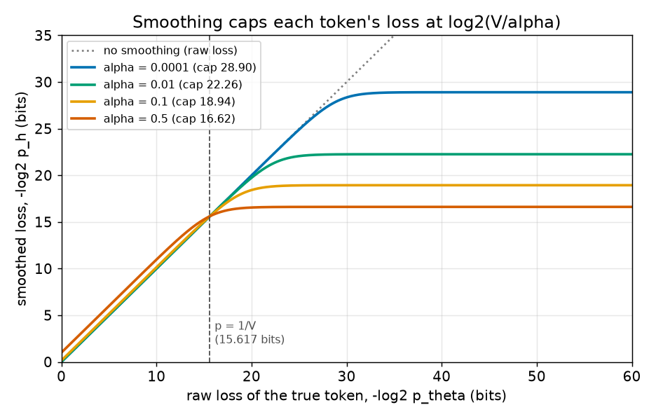
The figure shows the whole picture for one token: smoothing is a soft clamp. Left of the dashed line (\(p_\theta > 1/V\)) it adds a small premium; right of it (\(p_\theta < 1/V\)) it lowers the loss, flattening it to the ceiling.
Step 3 — checking Theorem A.2 numerically¶
The script draws 1,000,007 values of \(p_\theta\) in \((0,1)\) for each of the 8 values of \(\alpha\): half uniform, half spread evenly over the exponents from \(10^{-300}\) to 1, plus extremes from \(5\times10^{-324}\) (the smallest positive float64) to \(1 - 1.1\times10^{-16}\) (script section [3]).
- Smoothed losses outside \([\text{lower end}, \text{upper end}]\): 0.
- Float64 results landing exactly on an endpoint: 3,712,326. These are rounding: for \(p_\theta = 10^{-300}\), \((1-\alpha)p_\theta + \alpha/V\) is \(\alpha/V\) to every printed digit.
- Computing the distances to the ends with a numerically stable formula (
log1p) shows they are all positive: the smallest distance to the upper end is \(3.582\times10^{-319}\) bits, to the lower end \(1.602\times10^{-16}\) bits. In exact arithmetic the interval is open, as Theorem A.2 says. - With \(p_\theta = 0\) exactly, the loss equals the upper end; with \(p_\theta = 1\) it equals the lower end. So the closed interval is the one that holds for any value a computer can produce (erratum E13).
Step 4 — checking the properties¶
Script section [4]:
- Property 1. Over all samples and all 8 values of \(\alpha\), the largest value of smoothed loss \(-\) raw loss \(- \log_2\frac{1}{1-\alpha}\) is \(-2.871\times10^{-9}\) bits, never positive.
- Property 3. For 40 random next-token distributions over all 50,257 tokens and 8 values of \(\alpha\), the top-1, top-10 and top-100 sets were unchanged in 960 of 960 cases.
- Property 4. For the uniform model, the smoothed loss is 15.617037 bits for every \(\alpha\), equal to \(\log_2 V\).
Step 5 — the trade-off on a toy model¶
To see the trade-off with a model whose every number we know, the script builds a toy "trained model" (script section [6]). It has 10,000 documents of 200 tokens. For each token it draws the base probability of the real token: 80 % of tokens are ordinary (surprisal drawn from a Gamma distribution with mean 7 bits), 18 % are hard (surprisal uniform between 12 and 30 bits), and 2 % are catastrophic (\(p_\theta = 10^{-12}\)). Its unsmoothed BPD is 10.1807 bits per token, and 21.44 % of its tokens have \(p_\theta < 1/V\).
For the bound we use Eq. (1) with a compressed size of 20 KB plus 3 bits to name \(\alpha\), \(m = 8{,}009{,}762\)
documents [SOURCE: nanoGPT prepare.py / authors' code, erratum E32] and \(\delta = 0.05\) SOURCE: authors'
code, erratum E31, 1 KB = 8,192 bits (erratum E35). We treat the toy's 10,000-document average as if it were the
average over all \(m\) training documents; Chapter 17 adds the correction for estimating it on a
subsample, a second term that is also proportional to \(\Delta\). The complexity term is then \(0.08421\times\Delta\).
| \(\alpha\) | smoothed empirical risk | \(\Delta\) | complexity term | bound |
|---|---|---|---|---|
| 0.0001 | 9.9195 | 28.9046 | 2.4340 | 12.3535 |
| 0.001 | 9.7416 | 25.5814 | 2.1542 | 11.8957 |
| 0.005 | 9.5519 | 23.2537 | 1.9581 | 11.5101 |
| 0.01 | 9.4544 | 22.2464 | 1.8733 | 11.3277 |
| 0.05 | 9.2122 | 19.8650 | 1.6728 | 10.8850 |
| 0.1 | 9.1260 | 18.7870 | 1.5820 | 10.7080 |
| 0.25 | 9.1118 | 17.2020 | 1.4485 | 10.5603 |
| 0.5 | 9.3707 | 15.6171 | 1.3151 | 10.6858 |
(all in bits per token)
- The bound has a sweet spot. On the grid the best value is \(\alpha = 0.25\) (bound 10.5603). On a fine grid the minimum is at \(\alpha = 0.258\) (10.5590): the grid loses almost nothing.
- The empirical risk first falls. It drops from 9.9195 at \(\alpha = 0.0001\) to a minimum of 9.0955 at \(\alpha = 0.199\), below even the unsmoothed 10.1807, then rises. This is property 6 at work: the 21.44 % of tokens below \(1/V\) get cheaper.
- The bound prefers a larger α than the risk does (0.258 versus 0.199), because a larger \(\alpha\) also narrows \(\Delta\).
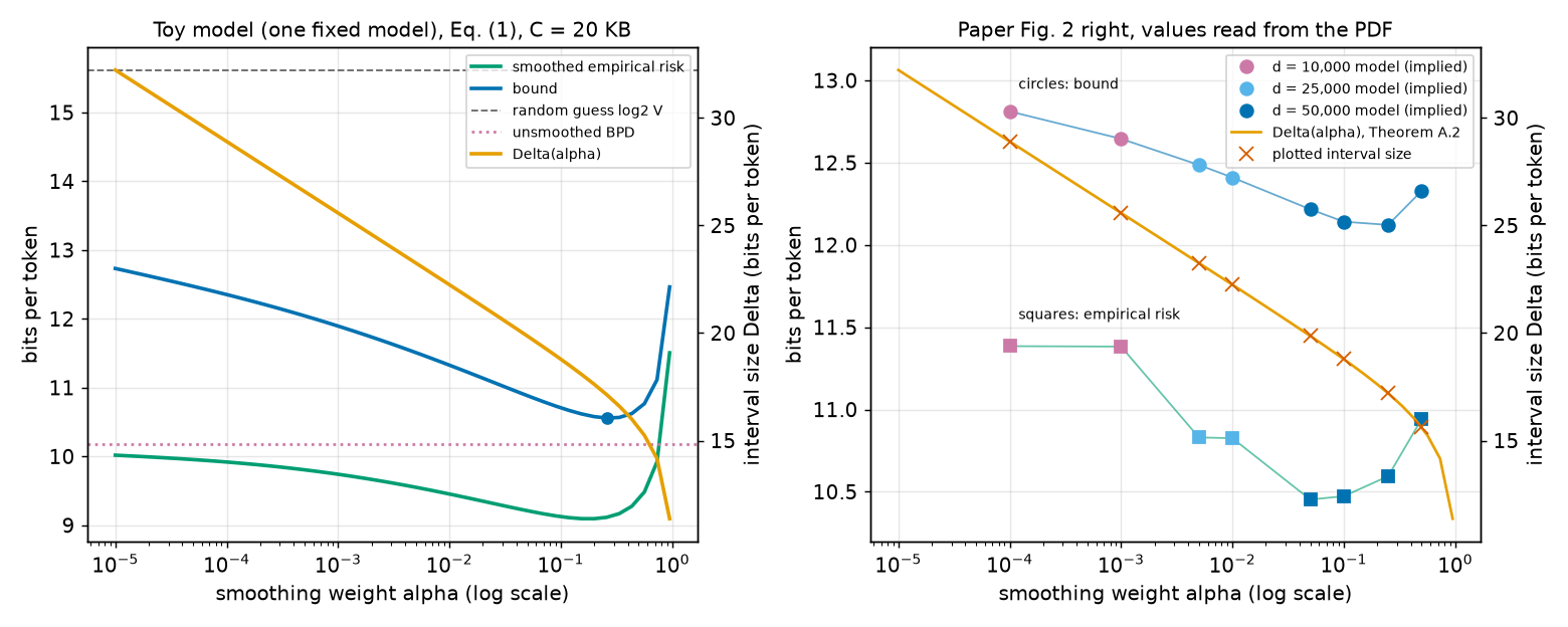
Step 6 — what Figure 2 (right) shows¶
PAPER Fig. 2 right and §4.3, p. 5 The paper's Figure 2 (right) plots, against \(\alpha\), the interval size, the
empirical risk and the bound, and says that the empirical risk goes up as \(\alpha\) grows. Read from the PDF
(fig_extract.py), the empirical risk is 11.3853, 11.3828, 10.8304, 10.8257, 10.4528, 10.4732, 10.5945 and 10.9417
bits per token at the eight grid values (script section [7]): it falls from 11.3853 to 10.4528 before rising.
Paper erratum E25: Figure 2 (right) has no tick labels on its bits-per-token axis
PAPER Fig. 2, p. 5 Only the interval-size axis of the right panel is labelled. MY EXPLANATION The
values above come from fig_extract.py, which reads the axis through gridlines shared with the left panel
(an inference). The inference is supported by the \(\alpha = 0.25\) point: empirical risk 10.5945 and bound
12.1224 are exactly the left panel's best model and Table 1's 12.12.
The script can say more, because the bound has the form \(\hat R + \Delta(\alpha)\,K\). Here the paper uses Eq. (3), the version of Eq. (1) that estimates the training loss on \(n = 10{,}000\) random documents (Chapter 17); both of its terms are \(\Delta\) times a number that depends on the compressed size but not on \(\alpha\). So for a single model, \(K = (\text{bound} - \text{empirical risk})/\Delta(\alpha)\) must be the same at every \(\alpha\). It is not:
| \(\alpha\) | empirical risk | bound | \(K\) | implied compressed size | matches Fig. 2 (left) |
|---|---|---|---|---|---|
| 0.0001 | 11.3853 | 12.8122 | 0.049367 | 3.883 KB | \(d\) = 10,000 (3.8782 KB) |
| 0.001 | 11.3828 | 12.6457 | 0.049367 | 3.883 KB | \(d\) = 10,000 |
| 0.005 | 10.8304 | 12.4868 | 0.071235 | 9.813 KB | \(d\) = 25,000 (9.8081 KB) |
| 0.01 | 10.8257 | 12.4104 | 0.071235 | 9.813 KB | \(d\) = 25,000 |
| 0.05 | 10.4528 | 12.2172 | 0.088817 | 16.537 KB | \(d\) = 50,000 (16.5325 KB) |
| 0.1 | 10.4732 | 12.1418 | 0.088817 | 16.537 KB | \(d\) = 50,000 |
| 0.25 | 10.5945 | 12.1224 | 0.088817 | 16.537 KB | \(d\) = 50,000 |
| 0.5 | 10.9417 | 12.3288 | 0.088817 | 16.537 KB | \(d\) = 50,000 |
(\(K\) is a pure number; the implied size solves Eq. (3) for \(C(h)\) with \(\delta = 0.05\), \(m = 8{,}009{,}762\), \(n = 10{,}000\) and no hyperparameter bits; \(d\) is the subspace dimension, the number of trained coordinates, which Chapter 18 defines.)
\(K\) takes exactly three values, and the compressed sizes they imply match three of the models in the left panel of Figure 2. The left panel's own eight points, by the same calculation, all use \(\Delta = 17.203\) to \(17.216\), i.e. \(\alpha = 0.25\), at every \(d\).
Paper erratum E41: Figure 2 (right) combines three different models
PAPER Fig. 2 and caption, p. 5 The caption presents the right panel as the interval size, empirical risk and bound as a function of \(\alpha\), adding that a different \(\alpha\) can be chosen for each model after training. The reader naturally takes the panel to show one trained model. MY EXPLANATION The plotted numbers say otherwise. The ratio (bound \(-\) empirical risk)\(/\Delta(\alpha)\) is constant for a single model but takes three values, which imply compressed sizes of 3.883, 9.813 and 16.537 KB: the \(d\) = 10,000, 25,000 and 50,000 models of the left panel. The points at \(\alpha = 0.0001, 0.001\) come from the first, \(0.005, 0.01\) from the second, and \(0.05\) to \(0.5\) from the third. An independent test (deeper block below) proves that no single model can produce the plotted empirical-risk curve: for one model, the drop from \(\alpha = 0.005\) to \(0.01\) would have to be at least 0.2307 bits, but the plot shows 0.0046. A plausible reading, which the paper does not state, is that each point is the best bound over \(d\) at that \(\alpha\): a large \(\Delta\) (small \(\alpha\)) makes complexity expensive and favours a smaller model. Consequence. Read as one model, the plotted empirical risk falls from 11.3853 to 10.4528 bits up to \(\alpha = 0.05\), which would contradict "the empirical risk goes up". That fall is a change of model, not an effect of smoothing (erratum E41). Within the one model that is plotted at four values (\(d\) = 50,000), the empirical risk only rises, 10.4528 → 10.4732 → 10.5945 → 10.9417, as the paper says. Smoothing can lower a weak model's empirical risk (Step 5 shows it in the toy), but Figure 2 does not show that. No reported bound changes; the figure is a less direct illustration of the trade-off than it appears.
Going deeper¶
Everything in this section is MY EXPLANATION.
Two deeper blocks sit next to the statements they support: "Proof of Theorem A.2, line by line" (under Theorem A.2) and "Proofs of the six properties" (under Properties of smoothing). Three more follow.
Going deeper: how the empirical risk can move with the mixing weight, and the single-model test
Setup. Fix one base model and the training documents. The empirical risk is a document-level average of per-token losses: \(\hat R(\alpha) = \sum_t w_t\,\ell_t(\alpha)\), where \(t\) runs over every token of every document, \(w_t = 1/(n L_j)\) for a token of document \(j\) (length \(L_j\), \(n\) documents), so \(w_t > 0\) and \(\sum_t w_t = 1\). Each \(\ell_t(\alpha) = -\log_2\big((1-\alpha)a_t + \alpha/V\big)\).
Shape of one token's loss on a log axis. Put \(u = \ln\alpha\), so \(\alpha = e^u\), and look at \(\ell\) as a function of \(u\) (the figure's log axis). By the chain rule, \(d\ell/du = \alpha\, d\ell/d\alpha = \frac{\alpha(a - 1/V)}{b\ln 2}\), with \(b = (1-\alpha)a + \alpha/V\).
- Bad token (\(a < 1/V\)). Write \(c = 1/V - a > 0\), so \(b = a + \alpha c\) and \(d\ell/du = -\frac{1}{\ln 2}\cdot\frac{\alpha c}{a + \alpha c} = -\frac{1}{\ln 2}\cdot\frac{1}{1 + a/(\alpha c)}\). As \(\alpha\) grows, \(a/(\alpha c)\) shrinks, so the fraction grows and the slope becomes more negative. A function whose slope keeps decreasing is concave. The slope lies between \(-1/\ln 2\) and 0 (bits per unit of \(\ln\alpha\)). Doubling \(\alpha\) moves \(u\) by \(\ln 2\), so the loss falls by at most 1 bit per doubling of \(\alpha\); for \(a \ll \alpha/V\) it falls by almost exactly 1 bit per doubling, because the loss is then close to \(\log_2(V/\alpha)\).
- Good token (\(a > 1/V\)). Write \(c' = a - 1/V > 0\), so \(b = a - \alpha c'\) and \(d\ell/du = \frac{1}{\ln 2}\cdot\frac{\alpha c'}{a - \alpha c'}\), positive and increasing in \(\alpha\): the loss is increasing and convex in \(u\).
So \(\hat R = B + G\), where \(B\) (weighted sum over bad tokens) is non-increasing and concave in \(u\), and \(G\) (the rest) is non-decreasing and convex in \(u\). This explains the toy's curve: \(B\) dominates at small \(\alpha\) (risk falls), \(G\) at large \(\alpha\) (risk rises).
How fast can good tokens get worse? Between \(\alpha_2 < \alpha_3\), a good token's loss rises by \(\log_2\frac{a - \alpha_2 c'}{a - \alpha_3 c'} = \log_2\frac{1 - \alpha_2 x}{1 - \alpha_3 x}\) with \(x = c'/a \in [0, 1)\). This increases with \(x\) (its derivative in \(x\) has the sign of \(\alpha_3 - \alpha_2 > 0\)), so it is less than \(\log_2\frac{1-\alpha_2}{1-\alpha_3}\). As the weights add up to at most 1, \(G(\alpha_3) - G(\alpha_2) \le \log_2\frac{1-\alpha_2}{1-\alpha_3}\).
The test. Take three values \(\alpha_1 < \alpha_2 < \alpha_3\) and \(\rho = \ln(\alpha_3/\alpha_2)/\ln(\alpha_2/\alpha_1)\), the ratio of the two steps on the log axis. A concave function's average slope can only decrease from one interval to the next, so \(B(\alpha_3) - B(\alpha_2) \le \rho\,\big(B(\alpha_2) - B(\alpha_1)\big)\). Since \(G\) does not decrease, \(B(\alpha_2) - B(\alpha_1) \le \hat R(\alpha_2) - \hat R(\alpha_1)\). Putting these together:
Any single model must satisfy this for every triple. The script checks it on Figure 2's eight points (script section [7]). Two triples fail:
- \((0.001, 0.005, 0.01)\): one model allows at most \(0.4307 \times (-0.5524) + 0.0073 = -0.2307\) bits; the plot shows \(-0.0046\).
- \((0.01, 0.05, 0.1)\): at most \(0.4307 \times (-0.3729) + 0.0780 = -0.0826\) bits; the plot shows \(+0.0203\).
In words: once the risk has dropped by 0.5524 bits between \(\alpha = 0.001\) and \(0.005\), the bad tokens responsible keep dragging it down at least as fast per doubling; it cannot level off at once. Both failing triples straddle a change of \(K\) in the table of Step 6, as the three-model reading predicts.
Going deeper: mixing per token versus mixing per document
PAPER §4.3, p. 5 The paper reports, as an empirical finding, that the token-level mixture gave better bounds than a mixture at the document level. MY EXPLANATION Here is why that is plausible.
Document-level mixture. For documents of a fixed length \(L\), mix whole-document probabilities: \(p_{\text{doc}}(X) = (1-\alpha)\,p_\theta(X) + \alpha V^{-L}\), where \(V^{-L}\) is the uniform distribution over the \(V^L\) documents of length \(L\). Its BPD is \(-\log_2 p_{\text{doc}}(X)/L\). The same two steps as in Theorem A.2 give
- If all documents had the same length \(L = 200\), this width is small: 15.683 bits at \(\alpha = 0.0001\) versus the token-level 28.905 (script section [6]).
- If documents can be as short as 1 token, the upper end is \(\log_2(V/\alpha)\) (at \(L = 1\)), and for long documents the lower end approaches 0. The width over all lengths is then \(\log_2(V/\alpha)\), slightly more than the token-level \(\Delta(\alpha)\): 17.617 versus 17.202 at \(\alpha = 0.25\).
Where token-level mixing wins: the empirical risk. A document-level mixture only helps documents whose whole average loss is worse than uniform guessing. A document with a few catastrophic tokens and many good ones gains nothing: in the toy, the document-level empirical risk stays at 10.1807–10.1828 bits (the unsmoothed BPD), while token-level smoothing caps each catastrophic token and reaches 9.9195, 9.4544 and 9.1118 at \(\alpha = 0.0001\), 0.01 and 0.25.
Net effect in the toy (bounds in bits per token, same complexity term): token-level 12.353 / 11.328 / 10.560; document-level with all lengths 200: 11.501 / 11.499 / 11.499; document-level with any length: 12.615 / 12.055 / 11.666, at \(\alpha = 0.0001\) / 0.01 / 0.25. The fixed-length document mixture wins at small \(\alpha\), but the best bound overall is token-level, 10.560 at \(\alpha = 0.25\). The paper's finding is an empirical statement about OpenWebText models; this toy shows only that it is the expected outcome when a model's errors are concentrated in a minority of tokens.
Going deeper: what the smoothed bound means, and what it would take to do better
What is certified. With probability at least \(1-\delta\) over the draw of the training documents (the model family, prior, grid, \(\delta\) and the widths \(\Delta(\alpha)\) fixed in advance), the expected per-document BPD of the smoothed, compressed model \(p_{\hat h}\) on a fresh document is at most the bound. It is a statement about that model only: it does not bound the unsmoothed model (property 2), and it is not a bound on token-level cross-entropy or perplexity (erratum E28, Chapter 6).
Why Δ matters so much. The complexity term is \(\Delta\) times a quantity that does not depend on the loss. At the paper's best setting, \(\Delta(0.25) = 17.2020\) bits per token multiplies a term of about 0.0888 (Step 6). A loss in \([0,1]\) with the same compressed size would pay 17.2 times less.
Could a smaller range be used? Theorem A.2's interval is tight for an arbitrary base model (proof block). Two routes could do better, neither used in the paper. (a) Bounds that use the variance of the loss instead of its range (Bernstein-type inequalities: like Hoeffding's, but with a deviation term driven mainly by the loss's standard deviation) pay little for rare extreme values; with smoothing, extreme values are rare. (b) A loss interval narrower than \([\text{lower end}, \text{upper end}]\) can be used if it is justified before the data, for example by a property of the architecture; one may not read it off the training data.
Choosing the base point of the interval. Hoeffding's inequality (Chapter 9) needs only the width, not where the interval sits. That is why the lower end, though positive, does not appear in the bound.
Common misconceptions¶
Everything in this section is MY EXPLANATION.
- Misconception: The paper's BPD bound of 12.12 bits per token bounds the GPT-2-style model's ordinary log-loss. — Actually: it bounds the smoothed model \(p_h\). The unsmoothed model's expected BPD can be larger by any amount (property 2); only the reverse direction is controlled (property 1).
- Misconception: Smoothing always makes the training loss worse. — Actually: tokens the model gave less than \(1/V\) get cheaper. In the toy model, the empirical risk falls from 9.9195 bits at \(\alpha = 0.0001\) to 9.0955 at \(\alpha = 0.199\), below the unsmoothed 10.1807. For good models the premium dominates.
- Misconception: Prediction smoothing is label smoothing. — Actually: label smoothing softens the training targets and changes \(\theta\); prediction smoothing mixes the outputs after training and does not touch \(\theta\). Only the latter guarantees the floor \(\alpha/V\) and hence a bounded loss.
- Misconception: The top-k error bounds also depend on \(\alpha\) and use \(\Delta(\alpha)\). — Actually: smoothing never changes which tokens are in the top k (property 3), so top-k error is the same with or without it, and its interval is \([0,1]\), \(\Delta = 1\).
- Misconception: Choosing \(\alpha\) after training is free. — Actually: each \(\alpha\) is a different hypothesis; naming one of the 8 grid values costs 3 bits in the prior, and the subsample-based choice raises the separate issue of erratum E07 (Chapter 17).
- Misconception: With \(\alpha = 0.5\) the loss range is small. — Actually: \(\Delta(0.5) = \log_2(V+1)\), a hair above the random-guess level 15.617 bits. On the paper's whole grid the width is at least that.
Self-test¶
Q1. Take \(\alpha = 0.05\) and \(V = 50{,}257\). (a) Give the interval of Theorem A.2 and its width. (b) A token gets base probability \(10^{-6}\): what are its raw and smoothed losses? (c) A token gets base probability 0.9: same question. Check (c) against property 1.
Answer
(a) Upper end \(\log_2(V/0.05) = 19.9390\) bits; width \(\Delta = \log_2(1 + 0.95V/0.05) = 19.8650\) bits; lower end \(19.9390 - 19.8650 = 0.0740\) bits (script line [Q1]).
(b) Raw: \(-\log_2 10^{-6} = 19.9316\) bits. Smoothed: \(-\log_2(0.95\times10^{-6} + 0.05/50{,}257) = 18.9719\) bits. The base probability \(10^{-6}\) is below \(1/V \approx 2\times10^{-5}\), so smoothing lowers the loss (property 6), here by about 1 bit, because the uniform share \(0.05/V\) is about the same size as \(0.95\times10^{-6}\) and the two add up.
(c) Raw: \(-\log_2 0.9 = 0.1520\) bits. Smoothed: 0.2260 bits. The increase, 0.0740 bits, is within the premium cap \(\log_2\frac{1}{1-0.05}\), which equals the lower end 0.0740 to four decimals.
Q2. A colleague says: "The paper certifies 12.12 bits per token for its model, and smoothing only ever adds at most \(\log_2\frac{1}{1-\alpha}\) bits, so the unsmoothed model must be within 0.415 bits of that." What is wrong?
Answer
The direction. Property 1 says smoothed loss \(\le\) raw loss \(+ \log_2\frac{1}{1-\alpha}\), i.e. the raw loss is at least the smoothed loss minus the premium. That turns an upper bound on the raw model into one on the smoothed model, not the other way round. A token with \(p_\theta = 0\) has infinite raw loss and smoothed loss \(\log_2(V/\alpha)\) (17.6170 bits at \(\alpha = 0.25\), Step 1), so the raw model's expected BPD can be infinite while the smoothed model's bound stays at 12.12. The certificate is about \(p_h\) only. (The colleague's 0.415 is the premium cap at \(\alpha = 0.25\), which equals the lower end 0.4150 in Step 1's table to four decimals.)
Q3. Why not choose \(\alpha = 0.9\), whose width \(\Delta = 12.4474\) bits is below \(\log_2 V\)? And why does the paper's grid stop at 0.5?
Answer
At \(\alpha = 0.9\) the interval is \((3.3217, 15.7690)\) (Step 1): every token costs at least 3.3217 bits, even a perfectly predicted one, and a good model pays a premium of up to \(\log_2\frac{1}{1-0.9} = 3.3219\) bits per token (property 1). The empirical risk therefore rises sharply, as the toy's curve near \(\alpha = 1\) shows (Step 5 figure). What is gained: relative to \(\alpha = 0.5\) the width is smaller by 3.1697 bits; with the paper's \(K = 0.088817\) for its best model (Step 6) the complexity term shrinks by only 0.2815 bits per token (script line [Q3]), far less than the premium. In general, beyond \(\alpha = 0.5\) the width falls slowly while the premium (at least about 1 bit at \(\alpha = 0.5\), growing without limit as \(\alpha \to 1\)) rises quickly, so for models whose loss is mostly on well-predicted tokens the optimum lies at or below 0.5. The paper does not justify its grid; this is our reading.
Code for this chapter¶
Run it from the project root:
.venv/Scripts/python explainer/code/ch16_smoothing.py
It reads the Figure 2 data written by explainer/code/fig_extract.py (outputs/fig_extract.json), runs in about
10 seconds, and writes the two figures above.
Source: ch16_smoothing.py
"""Chapter 16 demo: prediction smoothing and Theorem A.2.

Claims reproduced / illustrated
  * Paper §4.3, p. 5, Eq. (2): p_h = (1 - alpha) p_theta + alpha / V (token-level mixture with the uniform
    distribution); V = 50,257 [SOURCE: GPT-2 tokenizer; never printed in the paper, erratum E36].
  * Theorem A.2 (App. A.2, pp. 13-14, Eq. 7): every per-token smoothed loss, hence every document BPD, lies in
    (log2(V/alpha) - Delta, log2(V/alpha)) with Delta = log2(1 + (1 - alpha) V / alpha). Checked on the App. E
    alpha grid (p. 17) for 1,000,000 random p_theta values per alpha plus extremes; endpoints and strictness
    (erratum E13) checked with numerically stable formulas.
  * Table 1 (p. 7) random-guess BPD 15.62 = log2 V; Delta(0.5) = log2(V + 1).
  * Fig. 2 right (p. 5): the plotted "worst case interval size" equals Delta(alpha) (data read from the PDF by
    fig_extract.py).
  * [MY ANALYSIS] Properties: smoothed loss <= raw loss + log2(1/(1-alpha)); top-k sets unchanged; uniform model
    unchanged with BPD log2 V; Delta(alpha) >= log2(V+1) for alpha <= 0.5.
  * [MY ANALYSIS] Smoothing trade-off on a toy model (analogue of Fig. 2 right) with Eq. (1), C = 20 KB
    (1 KB = 8192 bits, erratum E35), m = 8,009,762 [SOURCE nanoGPT / authors' code, E32], delta = 0.05
    [SOURCE authors' code, E31]; token-level vs document-level mixing.
  * [MY ANALYSIS] Fig. 2 right audit: (bound - empirical risk) / Delta takes three different values, so the
    eight alpha points come from three different compressed sizes; a concavity argument shows the plotted
    empirical-risk curve cannot come from one fixed model (new erratum, logged in work/errata_parts/16.md).

Outputs: code/outputs/ch16_smoothing.txt, docs/assets/fig/ch16_clamp.png, docs/assets/fig/ch16_alpha_tradeoff.png
"""
from __future__ import annotations

import json
import math
import sys
import time
from pathlib import Path

import numpy as np
from scipy.optimize import brentq

import matplotlib
matplotlib.use("Agg")
import matplotlib.pyplot as plt

HERE = Path(__file__).resolve().parent
sys.path.insert(0, str(HERE))
import pacbound as pb  # noqa: E402

OUT_TXT = HERE / "outputs" / "ch16_smoothing.txt"
FIG_DIR = HERE.parent / "docs" / "assets" / "fig"
FIG_CLAMP = FIG_DIR / "ch16_clamp.png"
FIG_TRADE = FIG_DIR / "ch16_alpha_tradeoff.png"
FIG_JSON = HERE / "outputs" / "fig_extract.json"

T0 = time.time()
LINES: list[str] = []


def out(s: str = "") -> None:
    print(s)
    LINES.append(s)


V = pb.V_GPT2
LOG2V = pb.random_guess_bpd(V)
GRID = pb.ALPHA_GRID
LN2 = pb.LN2


def smoothed_loss(p, alpha):
    """Per-token smoothed loss -log2((1-alpha) p + alpha/V), bits/token (vectorised)."""
    return -np.log2((1.0 - alpha) * p + alpha / V)


def gap_to_hi(p, alpha):
    """log2(V/alpha) - smoothed loss = log2(1 + (1-alpha) p V / alpha), computed with log1p (bits)."""
    return np.log1p(p * ((1.0 - alpha) * V / alpha)) / LN2


def gap_to_lo(p, alpha):
    """smoothed loss - lower end = -log2(1 - (1-alpha)(1-p) / ((1-alpha) + alpha/V)), via log1p (bits)."""
    return -np.log1p(-(1.0 - alpha) * (1.0 - p) / ((1.0 - alpha) + alpha / V)) / LN2


out("Chapter 16 - prediction smoothing  (ch16_smoothing.py, seed 0)")

# ---------------------------------------------------------------------------
# [1] Constants and the random-guess level
# ---------------------------------------------------------------------------
out("[1] V = 50,257 [SOURCE: GPT-2 tokenizer]; units: bits per token throughout")
d05 = pb.smoothing_interval(0.5)[2]
out(f"    log2 V = {LOG2V:.4f} (Table 1 random guess 15.62, diff {15.62 - LOG2V:+.4f});"
    f"  Delta(0.5) = {d05:.6f} = log2(V+1) = {math.log2(V + 1):.6f}")
assert round(LOG2V, 2) == 15.62 and f"{LOG2V:.3f}" == "15.617"
assert abs(d05 - math.log2(V + 1)) < 1e-12

# ---------------------------------------------------------------------------
# [2] Theorem A.2 on the App. E grid, vs the Delta values plotted in Fig. 2 right
# ---------------------------------------------------------------------------
fig2 = json.loads(FIG_JSON.read_text(encoding="utf-8"))["figure2"]["right"]
pap_alpha = [round(e["alpha"], 4) for e in fig2["empirical_risk"]]
pap_emp = np.array([e["value"] for e in fig2["empirical_risk"]])
pap_bound = np.array([e["value"] for e in fig2["bound"]])
pap_delta = np.array([e["value"] for e in fig2["worst_case_interval"]])
assert pap_alpha == GRID

out("[2] Theorem A.2 interval (lo, hi), hi = log2(V/alpha), Delta = log2(1+(1-alpha)V/alpha), vs Fig. 2 right")
out("     alpha       lo        hi      Delta   Fig.2 Delta    diff   Delta-log2V")
for a, dp in zip(GRID, pap_delta):
    lo, hi, D = pb.smoothing_interval(a)
    out(f"    {a:<7g} {lo:8.4f} {hi:9.4f} {D:9.4f} {dp:11.4f} {dp - D:+9.5f} {D - LOG2V:10.5f}")
    assert abs(dp - D) < 5e-4          # plotted to 3 decimals
    assert D >= math.log2(V + 1) - 1e-12 and abs(hi - lo - D) < 1e-12   # property (v)
lo9, hi9, D9 = pb.smoothing_interval(0.9)
lo99, hi99, D99 = pb.smoothing_interval(0.99)
out(f"    outside the grid: alpha 0.9: ({lo9:.4f}, {hi9:.4f}), Delta {D9:.4f}; alpha 0.99: ({lo99:.4f}, {hi99:.4f}),"
    f" Delta {D99:.4f} (Delta -> 0 as alpha -> 1)")

# ---------------------------------------------------------------------------
# [3] Numeric check of Theorem A.2: 1,000,000 random p per alpha + extremes
# ---------------------------------------------------------------------------
rng = np.random.default_rng(0)
NP = 1_000_000
p_rand = np.concatenate([rng.random(NP // 2),                                  # uniform on (0,1)
                         10.0 ** rng.uniform(-300.0, 0.0, NP // 2)])           # log-uniform 1e-300..1
extremes = np.array([5e-324, 1e-300, 1e-12, 1.0 / V, 0.5, 1.0 - 1e-12, np.nextafter(1.0, 0.0)])
p_all = np.concatenate([p_rand, extremes])
p_all = p_all[(p_all > 0) & (p_all < 1)]
viol, at_end, min_ghi, min_glo = 0, 0, np.inf, np.inf
slack_i = -np.inf
for a in GRID:
    lo, hi, D = pb.smoothing_interval(a)
    L = smoothed_loss(p_all, a)
    viol += int(np.sum((L < lo - 1e-12) | (L > hi + 1e-12)))
    at_end += int(np.sum((L == hi) | (L == lo)))
    ghi, glo = gap_to_hi(p_all, a), gap_to_lo(p_all, a)
    assert np.all(ghi > 0) and np.all(glo > 0)
    min_ghi, min_glo = min(min_ghi, ghi.min()), min(min_glo, glo.min())
    # property (i): smoothed <= raw + log2(1/(1-alpha))
    raw = -np.log2(p_all)
    slack_i = max(slack_i, float(np.max(L - raw - math.log2(1.0 / (1.0 - a)))))
out(f"[3] {len(p_all):,} values of p_theta in (0,1) per alpha (uniform, log-uniform down to 1e-300, extremes"
    f" 5e-324 ... 1-1.1e-16), 8 alphas")
out(f"    outside [lo, hi]: {viol};  float64 results landing exactly on an endpoint: {at_end:,}"
    f" (rounding, e.g. p = 1e-300)")
out(f"    exact gaps (log1p): smallest distance to hi {min_ghi:.3e} bits, to lo {min_glo:.3e} bits -> strict, both > 0")
assert viol == 0
L0 = [float(smoothed_loss(0.0, a)) for a in GRID]
L1 = [float(smoothed_loss(1.0, a)) for a in GRID]
ok0 = all(abs(x - pb.smoothing_interval(a)[1]) < 1e-12 for x, a in zip(L0, GRID))
ok1 = all(abs(x - pb.smoothing_interval(a)[0]) < 1e-12 for x, a in zip(L1, GRID))
out(f"    p_theta = 0 gives exactly hi: {ok0};  p_theta = 1 gives exactly lo: {ok1} (closed interval, E13)")
assert ok0 and ok1

# ---------------------------------------------------------------------------
# [4] Properties (i), (iii), (iv)
# ---------------------------------------------------------------------------
out("[4] Properties [MY ANALYSIS]")
out(f"    (i) max over all samples of smoothed - raw - log2(1/(1-alpha)) = {slack_i:.3e} bits (<= 0)")
assert slack_i <= 1e-9
rng_k = np.random.default_rng(1)
same, total = 0, 0


def top100(q):
    """Indices of the 100 largest entries of q, in decreasing order of q."""
    idx = np.argpartition(-q, 100)[:100]
    return idx[np.argsort(-q[idx], kind="stable")]


for _ in range(40):
    z = rng_k.normal(0.0, 3.0, V)
    p = np.exp(z - z.max())
    p /= p.sum()
    top = top100(p)
    for a in GRID:
        ph = (1 - a) * p + a / V
        top_h = top100(ph)
        for k in (1, 10, 100):
            total += 1
            same += int(set(top[:k]) == set(top_h[:k]))
out(f"    (iii) top-k sets (k = 1, 10, 100) unchanged in {same}/{total} cases (40 random softmax distributions"
    f" over V, 8 alphas)")
assert same == total
uni = [float(smoothed_loss(1.0 / V, a)) for a in GRID]
out(f"    (iv) uniform p_theta = 1/V: smoothed loss = {min(uni):.6f} .. {max(uni):.6f} for every alpha"
      f" = log2 V = {LOG2V:.6f}")
assert max(abs(u - LOG2V) for u in uni) < 1e-9

# ---------------------------------------------------------------------------
# [5] Worked example: three tokens
# ---------------------------------------------------------------------------
out("[5] Three tokens (raw loss -log2 p_theta -> smoothed loss), bits")
for p in (1e-12, 0.5, 1.0 / V):
    row = "  ".join(f"a={a}: {float(smoothed_loss(p, a)):7.4f}" for a in (1e-4, 0.1, 0.5))
    out(f"    p = {p:<9.3g} raw {-math.log2(p):7.4f} | {row}")
out(f"    penalty cap log2(1/(1-alpha)): a=1e-4 {math.log2(1/(1-1e-4)):.6f}, a=0.1 {math.log2(1/0.9):.4f},"
    f" a=0.5 {math.log2(2):.4f}")

# ---------------------------------------------------------------------------
# [6] Toy trade-off (analogue of Fig. 2 right)
# ---------------------------------------------------------------------------
NDOC, LDOC = 10_000, 200
rng_t = np.random.default_rng(0)
NTOK = NDOC * LDOC
u = rng_t.random(NTOK)
s_bits = np.where(u < 0.80, rng_t.gamma(2.0, 3.5, NTOK),                  # ordinary tokens, mean 7 bits
                  np.where(u < 0.98, rng_t.uniform(12.0, 30.0, NTOK),    # hard tokens
                           -math.log2(1e-12)))                           # catastrophic: p = 1e-12
p_tok = np.exp2(-s_bits)
S_doc = s_bits.reshape(NDOC, LDOC).sum(axis=1)                            # raw NLL per document, bits
C_TOY = 20 * 8192                                                         # 20 KB, 1 KB = 8192 bits
HYP = math.log2(len(GRID))                                                # 3 bits to name alpha in the grid
lnP = pb.log_inv_prior_nats_from_bits(C_TOY, HYP)
K_toy = pb.eq1_complexity(lnP, pb.M_DOCS)                                 # complexity per unit of Delta


def emp_token(a):
    # all documents have LDOC tokens, so the mean of document means equals the mean over all tokens
    return float(smoothed_loss(p_tok, a).mean())


def emp_doc(a):
    # document-level mixture: p(X) = (1-a) 2^-S + a V^-L, per-token BPD = -log2 p(X) / L
    lp = np.logaddexp2(math.log2(1 - a) - S_doc, math.log2(a) - LDOC * LOG2V)
    return float((-lp / LDOC).mean())


raw_emp = float(s_bits.reshape(NDOC, LDOC).mean(axis=1).mean())
out(f"[6] Toy model [MY ANALYSIS]: {NDOC:,} docs x {LDOC} tokens; true-token surprisal: 80% Gamma(2, 3.5 bits),"
    f" 18% U[12,30] bits, 2% p=1e-12")
out(f"    unsmoothed BPD {raw_emp:.4f}; tokens with p_theta < 1/V: {np.mean(p_tok < 1 / V) * 100:.2f} %;"
    f" Eq.(1): C = 20 KB + log2 8 = 3 bits, m = 8,009,762, delta = 0.05 -> term = {K_toy:.5f} x Delta")
out("     alpha    emp risk   Delta    complexity   bound")
toy_rows = []
for a in GRID:
    D = pb.smoothing_interval(a)[2]
    e = emp_token(a)
    b = pb.eq1_bound(e, lnP, pb.M_DOCS, width=D)
    toy_rows.append((a, e, D, b))
    out(f"    {a:<7g} {e:9.4f} {D:9.4f} {K_toy * D:9.4f} {b:10.4f}")
best = min(toy_rows, key=lambda r: r[3])
fine = np.logspace(-5, math.log10(0.95), 45)
fine_emp = np.array([emp_token(a) for a in fine])
fine_D = np.array([pb.smoothing_interval(a)[2] for a in fine])
fine_bound = fine_emp + K_toy * fine_D
ib, ie = int(np.argmin(fine_bound)), int(np.argmin(fine_emp))
out(f"    best on grid: alpha = {best[0]} (bound {best[3]:.4f}); fine grid: bound min at alpha = {fine[ib]:.3f}"
    f" ({fine_bound[ib]:.4f}), emp-risk min at alpha = {fine[ie]:.3f} ({fine_emp[ie]:.4f})")

# token-level vs document-level mixing
out("    token- vs document-level mixing (same toy, same Eq. 1 term):")
for a in (1e-4, 0.01, 0.25):
    D = pb.smoothing_interval(a)[2]
    hiL = LOG2V + math.log2(1 / a) / LDOC
    loL = -math.log2((1 - a) + a * 2.0 ** (-LDOC * LOG2V)) / LDOC
    wL, wAny = hiL - loL, math.log2(V / a)
    et, ed = emp_token(a), emp_doc(a)
    out(f"    a={a:<6g} emp token {et:.4f} / doc {ed:.4f}; width token {D:.3f} / doc (all L=200) {wL:.3f}"
        f" / doc (any L>=1) {wAny:.3f}; bounds {et + K_toy * D:.3f} / {ed + K_toy * wL:.3f} / {ed + K_toy * wAny:.3f}")

# ---------------------------------------------------------------------------
# [7] Audit of Fig. 2 right [MY ANALYSIS]
# ---------------------------------------------------------------------------
fig2l = json.loads(FIG_JSON.read_text(encoding="utf-8"))["figure2"]["left"]
left_kb = [(round(e["d"], -2), e["value"]) for e in fig2l["compressed_size_kb"]]
n, m, dl = pb.N_SUB, pb.M_DOCS, pb.DELTA
s_ = n / (n + m)
t2_unit = math.sqrt(math.log(1 / ((1 - s_) * dl)) / (2 * n))
out("[7] Fig. 2 right audit: K = (bound - emp)/Delta; Eq. (3) => implied compressed size (no hyperparameter bits)")
out("     alpha    emp      bound    K         implied C (KB)  nearest Fig.2-left model")
Ks = []
for a, e, b, D in zip(GRID, pap_emp, pap_bound, pap_delta):
    K = (b - e) / pb.smoothing_interval(a)[2]
    t1 = K - t2_unit
    price = 2 * m * t1 * t1 - math.log(1 / (s_ * dl))
    C = brentq(lambda c: pb.log_inv_prior_nats_from_bits(c) - price, 2.0, 1e9)
    kb = C / 8192
    dnear, kbnear = min(left_kb, key=lambda r: abs(r[1] - kb))
    Ks.append(K)
    out(f"    {a:<7g} {e:7.4f} {b:8.4f} {K:.6f} {kb:10.3f}       d = {int(dnear):,} ({kbnear:.4f} KB)")
Ks = np.array(Ks)
groups = sorted(set(np.round(Ks, 4)))
out(f"    distinct K values: {len(groups)} -> {', '.join(f'{g:.4f}' for g in groups)}")
assert len(groups) == 3
# concavity test: for ONE fixed model, R(alpha3)-R(alpha2) <= rho (R(alpha2)-R(alpha1)) + log2((1-a2)/(1-a3))
viol_txt = []
for i in range(len(GRID) - 2):
    a1, a2, a3 = GRID[i], GRID[i + 1], GRID[i + 2]
    rho = math.log(a3 / a2) / math.log(a2 / a1)
    cap = rho * (pap_emp[i + 1] - pap_emp[i]) + math.log2((1 - a2) / (1 - a3))
    obs = pap_emp[i + 2] - pap_emp[i + 1]
    if obs > cap + 1e-9:
        viol_txt.append(f"({a1},{a2},{a3}): one model allows <= {rho:.4f} x ({pap_emp[i + 1] - pap_emp[i]:+.4f})"
                        f" + {math.log2((1 - a2) / (1 - a3)):.4f} = {cap:+.4f}, plotted {obs:+.4f}")
out(f"    single-model concavity test violated by {len(viol_txt)} triples: " + "; ".join(viol_txt))
assert len(viol_txt) >= 1
# Fig. 2 left: which Delta (hence which alpha) do its eight points use?
impl_D = []
for e, b, c in zip(fig2l["empirical_risk"], fig2l["bound"], fig2l["compressed_size_kb"]):
    t1, t2 = pb.eq3_terms(pb.log_inv_prior_nats_from_bits(c["value"] * 8192), m, n)
    impl_D.append((b["value"] - e["value"]) / (t1 + t2))
out(f"    Fig. 2 left (d sweep): implied Delta {min(impl_D):.3f} .. {max(impl_D):.3f} for all 8 d"
    f" -> alpha = 0.25 (Delta 17.202) at every d")
assert all(abs(x - pb.smoothing_interval(0.25)[2]) < 0.02 for x in impl_D)

# ---------------------------------------------------------------------------
# [Q] Self-test numbers
# ---------------------------------------------------------------------------
loq, hiq, Dq = pb.smoothing_interval(0.05)
out(f"[Q1] alpha = 0.05: lo {loq:.4f}, hi {hiq:.4f}, Delta {Dq:.4f}; token p = 1e-6: raw {-math.log2(1e-6):.4f},"
    f" smoothed {float(smoothed_loss(1e-6, 0.05)):.4f}; p = 0.9: raw {-math.log2(0.9):.4f},"
    f" smoothed {float(smoothed_loss(0.9, 0.05)):.4f} bits")
K50 = float(Ks[-1])
dsave = pb.smoothing_interval(0.5)[2] - pb.smoothing_interval(0.9)[2]
out(f"[Q3] alpha 0.9 vs 0.5: Delta smaller by {dsave:.4f}; x K = {K50:.6f} (Fig. 2, d = 50,000) -> {K50 * dsave:.4f}"
    f" bits/token saved; premium cap log2(1/(1-0.9)) = {math.log2(10):.4f} bits")

# ---------------------------------------------------------------------------
# Figures
# ---------------------------------------------------------------------------
FIG_DIR.mkdir(parents=True, exist_ok=True)
plt.rcParams.update({"font.size": 11})
cols = ["#0072B2", "#009E73", "#E69F00", "#D55E00"]

fig, ax = plt.subplots(figsize=(7.2, 4.6))
sgrid = np.linspace(0, 60, 600)
ax.plot(sgrid, sgrid, color="0.5", ls=":", lw=1.5, label="no smoothing (raw loss)")
for c, a in zip(cols, (1e-4, 0.01, 0.1, 0.5)):
    lo, hi, D = pb.smoothing_interval(a)
    ax.plot(sgrid, smoothed_loss(np.exp2(-sgrid), a), color=c, lw=2, label=f"alpha = {a:g} (cap {hi:.2f})")
ax.axvline(LOG2V, color="0.3", lw=1, ls="--")
ax.text(LOG2V + 0.5, 2, "p = 1/V\n(15.617 bits)", fontsize=9, color="0.3")
ax.set_xlabel("raw loss of the true token, -log2 p_theta (bits)")
ax.set_ylabel("smoothed loss, -log2 p_h (bits)")
ax.set_title("Smoothing caps each token's loss at log2(V/alpha)")
ax.set_xlim(0, 60)
ax.set_ylim(0, 35)
ax.legend(fontsize=9, loc="upper left")
ax.grid(alpha=0.3)
fig.tight_layout()
fig.savefig(FIG_CLAMP, dpi=130)
plt.close(fig)

fig, (axl, axr) = plt.subplots(1, 2, figsize=(12, 4.8))
for axx, title in ((axl, "Toy model (one fixed model), Eq. (1), C = 20 KB"),
                   (axr, "Paper Fig. 2 right, values read from the PDF")):
    axx.set_xscale("log")
    axx.set_xlabel("smoothing weight alpha (log scale)")
    axx.set_ylabel("bits per token")
    axx.set_title(title, fontsize=11)
    axx.grid(alpha=0.3)
axl.plot(fine, fine_emp, color="#009E73", lw=2, label="smoothed empirical risk")
axl.plot(fine, fine_bound, color="#0072B2", lw=2, label="bound")
axl.axhline(LOG2V, color="0.4", ls="--", lw=1, label="random guess log2 V")
axl.plot([fine[ib]], [fine_bound[ib]], "o", color="#0072B2")
axl.axhline(raw_emp, color="#CC79A7", ls=":", lw=1.5, label="unsmoothed BPD")
axl2 = axl.twinx()
axl2.plot(fine, fine_D, color="#E69F00", lw=2, label="Delta(alpha)")
axl2.set_ylabel("interval size Delta (bits per token)")
h1, l1 = axl.get_legend_handles_labels()
h2, l2 = axl2.get_legend_handles_labels()
axl.legend(h1 + h2, l1 + l2, fontsize=8, loc="upper right")
grp_col = {groups[0]: "#CC79A7", groups[1]: "#56B4E9", groups[2]: "#0072B2"}
grp_lab = {groups[0]: "d = 10,000 model", groups[1]: "d = 25,000 model", groups[2]: "d = 50,000 model"}
axr.plot(GRID, pap_emp, color="#009E73", lw=1, alpha=0.6)
axr.plot(GRID, pap_bound, color="#0072B2", lw=1, alpha=0.6)
for g in groups:
    idx = [i for i, K in enumerate(Ks) if round(K, 4) == g]
    axr.plot([GRID[i] for i in idx], pap_emp[idx], "s", color=grp_col[g], ms=7)
    axr.plot([GRID[i] for i in idx], pap_bound[idx], "o", color=grp_col[g], ms=7, label=grp_lab[g] + " (implied)")
axr.text(1.2e-4, 11.55, "squares: empirical risk", fontsize=8)
axr.text(1.2e-4, 12.95, "circles: bound", fontsize=8)
axr.set_ylim(10.2, 13.2)
axr2 = axr.twinx()
axr2.plot(fine, fine_D, color="#E69F00", lw=1.5, label="Delta(alpha), Theorem A.2")
axr2.plot(GRID, pap_delta, "x", color="#D55E00", ms=8, label="plotted interval size")
axr2.set_ylabel("interval size Delta (bits per token)")
h1, l1 = axr.get_legend_handles_labels()
h2, l2 = axr2.get_legend_handles_labels()
axr.legend(h1 + h2, l1 + l2, fontsize=8, loc="upper right")
fig.tight_layout()
fig.savefig(FIG_TRADE, dpi=130)
plt.close(fig)

out("figures: docs/assets/fig/ch16_clamp.png, docs/assets/fig/ch16_alpha_tradeoff.png; all assertions passed")
print(f"runtime {time.time() - T0:.1f} s (console only, so the output file is deterministic)")
OUT_TXT.parent.mkdir(parents=True, exist_ok=True)
OUT_TXT.write_text("\n".join(LINES) + "\n", encoding="utf-8")
Output:
Chapter 16 - prediction smoothing  (ch16_smoothing.py, seed 0)
[1] V = 50,257 [SOURCE: GPT-2 tokenizer]; units: bits per token throughout
    log2 V = 15.6170 (Table 1 random guess 15.62, diff +0.0030);  Delta(0.5) = 15.617066 = log2(V+1) = 15.617066
[2] Theorem A.2 interval (lo, hi), hi = log2(V/alpha), Delta = log2(1+(1-alpha)V/alpha), vs Fig. 2 right
     alpha       lo        hi      Delta   Fig.2 Delta    diff   Delta-log2V
    0.0001    0.0001   28.9047   28.9046     28.9045  -0.00006   13.28757
    0.001     0.0014   25.5828   25.5814     25.5813  -0.00006    9.96434
    0.005     0.0072   23.2609   23.2537     23.2536  -0.00006    7.63662
    0.01      0.0145   22.2609   22.2464     22.2463  -0.00006    6.62936
    0.05      0.0740   19.9390   19.8650     19.8649  -0.00006    4.24793
    0.1       0.1520   18.9390   18.7870     18.7869  -0.00005    3.16993
    0.25      0.4150   17.6170   17.2020     17.2020  -0.00005    1.58497
    0.5       1.0000   16.6170   15.6171     15.6170  -0.00005    0.00003
    outside the grid: alpha 0.9: (3.3217, 15.7690), Delta 12.4474; alpha 0.99: (6.6410, 15.6315), Delta 8.9905 (Delta -> 0 as alpha -> 1)
[3] 1,000,007 values of p_theta in (0,1) per alpha (uniform, log-uniform down to 1e-300, extremes 5e-324 ... 1-1.1e-16), 8 alphas
    outside [lo, hi]: 0;  float64 results landing exactly on an endpoint: 3,712,326 (rounding, e.g. p = 1e-300)
    exact gaps (log1p): smallest distance to hi 3.582e-319 bits, to lo 1.602e-16 bits -> strict, both > 0
    p_theta = 0 gives exactly hi: True;  p_theta = 1 gives exactly lo: True (closed interval, E13)
[4] Properties [MY ANALYSIS]
    (i) max over all samples of smoothed - raw - log2(1/(1-alpha)) = -2.871e-09 bits (<= 0)
    (iii) top-k sets (k = 1, 10, 100) unchanged in 960/960 cases (40 random softmax distributions over V, 8 alphas)
    (iv) uniform p_theta = 1/V: smoothed loss = 15.617037 .. 15.617037 for every alpha = log2 V = 15.617037
[5] Three tokens (raw loss -log2 p_theta -> smoothed loss), bits
    p = 1e-12     raw 39.8631 | a=0.0001: 28.9040  a=0.1: 18.9390  a=0.5: 16.6170
    p = 0.5       raw  1.0000 | a=0.0001:  1.0001  a=0.1:  1.1520  a=0.5:  1.9999
    p = 1.99e-05  raw 15.6170 | a=0.0001: 15.6170  a=0.1: 15.6170  a=0.5: 15.6170
    penalty cap log2(1/(1-alpha)): a=1e-4 0.000144, a=0.1 0.1520, a=0.5 1.0000
[6] Toy model [MY ANALYSIS]: 10,000 docs x 200 tokens; true-token surprisal: 80% Gamma(2, 3.5 bits), 18% U[12,30] bits, 2% p=1e-12
    unsmoothed BPD 10.1807; tokens with p_theta < 1/V: 21.44 %; Eq.(1): C = 20 KB + log2 8 = 3 bits, m = 8,009,762, delta = 0.05 -> term = 0.08421 x Delta
     alpha    emp risk   Delta    complexity   bound
    0.0001     9.9195   28.9046    2.4340    12.3535
    0.001      9.7416   25.5814    2.1542    11.8957
    0.005      9.5519   23.2537    1.9581    11.5101
    0.01       9.4544   22.2464    1.8733    11.3277
    0.05       9.2122   19.8650    1.6728    10.8850
    0.1        9.1260   18.7870    1.5820    10.7080
    0.25       9.1118   17.2020    1.4485    10.5603
    0.5        9.3707   15.6171    1.3151    10.6858
    best on grid: alpha = 0.25 (bound 10.5603); fine grid: bound min at alpha = 0.258 (10.5590), emp-risk min at alpha = 0.199 (9.0955)
    token- vs document-level mixing (same toy, same Eq. 1 term):
    a=0.0001 emp token 9.9195 / doc 10.1807; width token 28.905 / doc (all L=200) 15.683 / doc (any L>=1) 28.905; bounds 12.353 / 11.501 / 12.615
    a=0.01   emp token 9.4544 / doc 10.1808; width token 22.246 / doc (all L=200) 15.650 / doc (any L>=1) 22.261; bounds 11.328 / 11.499 / 12.055
    a=0.25   emp token 9.1118 / doc 10.1828; width token 17.202 / doc (all L=200) 15.625 / doc (any L>=1) 17.617; bounds 10.560 / 11.499 / 11.666
[7] Fig. 2 right audit: K = (bound - emp)/Delta; Eq. (3) => implied compressed size (no hyperparameter bits)
     alpha    emp      bound    K         implied C (KB)  nearest Fig.2-left model
    0.0001  11.3853  12.8122 0.049367      3.883       d = 10,000 (3.8782 KB)
    0.001   11.3828  12.6457 0.049367      3.883       d = 10,000 (3.8782 KB)
    0.005   10.8304  12.4868 0.071235      9.813       d = 25,000 (9.8081 KB)
    0.01    10.8257  12.4104 0.071235      9.813       d = 25,000 (9.8081 KB)
    0.05    10.4528  12.2172 0.088817     16.537       d = 50,000 (16.5325 KB)
    0.1     10.4732  12.1418 0.088817     16.537       d = 50,000 (16.5325 KB)
    0.25    10.5945  12.1224 0.088817     16.537       d = 50,000 (16.5325 KB)
    0.5     10.9417  12.3288 0.088817     16.537       d = 50,000 (16.5325 KB)
    distinct K values: 3 -> 0.0494, 0.0712, 0.0888
    single-model concavity test violated by 2 triples: (0.001,0.005,0.01): one model allows <= 0.4307 x (-0.5524) + 0.0073 = -0.2307, plotted -0.0046; (0.01,0.05,0.1): one model allows <= 0.4307 x (-0.3729) + 0.0780 = -0.0826, plotted +0.0203
    Fig. 2 left (d sweep): implied Delta 17.203 .. 17.216 for all 8 d -> alpha = 0.25 (Delta 17.202) at every d
[Q1] alpha = 0.05: lo 0.0740, hi 19.9390, Delta 19.8650; token p = 1e-6: raw 19.9316, smoothed 18.9719; p = 0.9: raw 0.1520, smoothed 0.2260 bits
[Q3] alpha 0.9 vs 0.5: Delta smaller by 3.1697; x K = 0.088817 (Fig. 2, d = 50,000) -> 0.2815 bits/token saved; premium cap log2(1/(1-0.9)) = 3.3219 bits
figures: docs/assets/fig/ch16_clamp.png, docs/assets/fig/ch16_alpha_tradeoff.png; all assertions passed