08. Linear-algebra toolkit¶
Where this fits
Prerequisites: Chapter 1 (random variable, independence, i.i.d., normal distribution, expectation, variance, conditional expectation, law of large numbers). Nothing else. Used later by: Chapter 5 (a transformer is mostly matrix products), Chapter 7 (training through \(\theta=\theta_0+Pw\)), Chapter 18 (random subspaces and the Kronecker projector), Chapter 19 (LoRA's low-rank update) and Chapter 20 (SubLoRA). Purpose: build, from zero, exactly the vector-and-matrix tools the paper uses to shrink a model, and prove every fact that later chapters lean on.
The problem this chapter solves¶
MY EXPLANATION A neural network stores what it has learned as a very long list of numbers, its parameters (the adjustable numbers inside a model; Chapter 2). The models in this paper have between about a hundred million and a billion of them.
The paper makes such a model compressible by letting only a few thousand numbers move during training. All the other numbers are tied to those few by a fixed rule. That rule is written in the language of vectors and matrices.
PAPER §3, p. 4 The background section describes "subspace training" from Lotfi et al. (2022). All \(D\) weights of the network, collected in one list \(\theta\), are written as a fixed random starting list \(\theta_0\) plus a matrix \(P\) times a much shorter list \(w\) of length \(d\): \(\theta=\theta_0+Pw\). The matrix \(P\) is built as a Kronecker product of two random Gaussian matrices and scaled so that \(P^\top P\approx I\). The same section describes LoRA, which writes a change to a weight matrix (a table of parameters inside the network) as the product of two thin matrices.
PAPER §5, p. 6 In the paper's own method, SubLoRA (which Chapter 20 explains), the projector is \(P=Q_1\otimes Q_2\), where \(Q_1\) and \(Q_2\) come from a QR factorization of Gaussian random matrices.
PAPER App. E, pp. 16–17 The short list \(w\) has length \(d\) of at most 200,000 in the experiments, and the LoRA "rank" \(r\) (a size defined later in this chapter) is 1 or 4 (output [4]).
MY EXPLANATION Every symbol in those sentences is linear algebra. This chapter answers six questions:
- What do \(Pw\) and \(\theta_0+Pw\) compute, and how much arithmetic does that take?
- What does \(P^\top P=I\) promise, and why would anyone want it?
- What is "low rank", and why does a product of two thin matrices need so few numbers?
- How does a QR factorization turn a random matrix into one with \(P^\top P=I\) exactly?
- What is a Kronecker product \(\otimes\), and why is a Kronecker-built \(P\) cheap to store and to use?
- Why does a plain random Gaussian matrix already satisfy \(P^\top P=I\) approximately?
How the paper trains through these tools is the job of Chapter 18 (subspaces) and Chapter 19 (LoRA). Here we only build the tools.
Intuition (and where the analogy breaks)¶
Everything in this section is MY EXPLANATION.
A matrix is a mixing machine. You feed in a list of numbers and get out another list. Each output number is a weighted sum of all the input numbers. Think of the inputs as amounts of ingredients and of each row of the matrix as one recipe: "take 1 part of ingredient one and 2 parts of ingredient two". Each output is one finished dish.
A matrix with orthonormal columns places a small world inside a big one without distortion. Hold a flat sheet of paper in a room. Every point on the sheet also has a place in the room. Distances measured along the sheet equal distances measured in the room. The sheet is a 2-dimensional world sitting inside a 3-dimensional one. A matrix with orthonormal columns does the same for a list of \(d\) numbers placed inside a list of \(D\) numbers.
Low rank means few ingredients. Look at a multiplication table. Every row is a multiple of the first row. You can rebuild the whole table from one row and one column. The rank of a table counts how many such independent ingredients it really needs.
A Kronecker product is a tiled floor. Take a small pattern, a tile. Lay a grid of tiles, where each tile is the pattern scaled by one number from a second small table. The whole floor is the Kronecker product of the two small tables.
Where it breaks:
- The mixing machine can only form weighted sums. Double the input and the output doubles. It cannot square a number or cut it off at zero. (Neural networks put such non-linear steps between matrices; Chapter 5.)
- The tiled floor suggests you must lay every tile, that is, store the whole big matrix, before you can use it. You never do. When the floor acts on a list, each output number mixes contributions from every tile in its row of tiles, so the tiles "overlap" in their effect. The efficient way to compute that effect (the vec trick, below) works with the two small tables and never builds the floor.
- The sheet-in-a-room picture is 3-dimensional. In thousands of dimensions geometry behaves differently: two directions chosen at random are almost always nearly perpendicular. No 3-D picture shows this. We prove it instead.
Precise definition¶
Everything in this section is standard mathematics and is MY EXPLANATION unless a paragraph carries another tag.
Letters used in this chapter
The explainer's notation table fixes some letters for the whole site: \(D\) and \(d\) are sizes, \(\theta\), \(\theta_0\), \(w\) and \(P\) are the parameter lists and the projector, \(B\) and \(A\) are the two LoRA factors, and \(r\) is a rank. For general matrices this chapter therefore uses other letters: \(W\) (any matrix), \(G\) (a Gaussian matrix), \(Q\) (a matrix with orthonormal columns), \(T\) (a triangular matrix) and \(M_1,M_2,N_1,N_2\) (inside Kronecker products). Textbooks often state the Kronecker rules with the letters \(A,B,C,D\); we avoid that because \(D\) is the parameter count.
Vectors and dimension¶
A vector is an ordered list of numbers. Example: \(v=(2,1)\). Order matters: \((2,1)\) and \((1,2)\) are different vectors.
The dimension of a vector is how many numbers it holds. The vector \((2,1)\) has dimension 2.
The set of all vectors of dimension \(b\) with real-number entries is written \(\mathbb R^b\). The symbol \(\in\) means "is a member of". So \(\theta\in\mathbb R^D\) says "\(\theta\) is a list of \(D\) real numbers". Entry number \(i\) of a vector \(v\) is written \(v_i\).
Two vectors of the same dimension are added entry by entry: \((2,1)+(1,3)=(3,4)\).
A single number is called a scalar. Multiplying a vector by a scalar multiplies every entry: \(3\cdot(2,1)=(6,3)\). The zero vector has every entry equal to 0.
We usually picture vectors as columns (written top to bottom). Writing them in a line, as above, means the same thing.
Matrices and shape¶
A matrix is a rectangular table of numbers. Its shape is "number of rows × number of columns". A matrix with \(a\) rows and \(b\) columns has shape \(a\times b\). The set of all such real matrices is \(\mathbb R^{a\times b}\). The entry in row \(i\) and column \(j\) of a matrix \(W\) is written \(W_{ij}\).
Example:
Each column of \(W\) is a vector in \(\mathbb R^3\). A vector in \(\mathbb R^b\) is the same thing as a \(b\times1\) matrix (a single column).
Matrix–vector product¶
If \(W\in\mathbb R^{a\times b}\) and \(v\in\mathbb R^b\), the matrix–vector product \(Wv\) is the vector in \(\mathbb R^a\) whose \(i\)-th entry is
The symbol \(\sum_{j=1}^{b}\) means "add up the term that follows for \(j=1,2,\dots,b\)". In words: walk along row \(i\) of \(W\), multiply each entry by the matching entry of \(v\), and add the results.
Example (output [1]): with the \(W\) above and \(v=(2,1)\), \(Wv=(1\cdot2+2\cdot1,\;3\cdot2+4\cdot1,\;5\cdot2+6\cdot1)=(4,10,16)\).
Shapes must fit: the number of columns of \(W\) must equal the dimension of \(v\).
Cost. Each of the \(a\) outputs needs \(b\) multiplications, so \(Wv\) costs \(a\cdot b\) multiplications (6 in the example). This count matters later. If \(P\) is \(D\times d\), computing \(Pw\) the plain way costs \(D\cdot d\) multiplications, and storing \(P\) takes \(D\cdot d\) numbers.
Column view. The same product is a weighted sum of the columns of \(W\), with the entries of \(v\) as the weights:
In general \(Wv=v_1\cdot(\text{column }1)+\dots+v_b\cdot(\text{column }b)\). This view is the key to rank, below.
Linearity. For any vectors \(v,v'\) and scalar \(c\): \(W(v+v')=Wv+Wv'\) and \(W(cv)=c\,Wv\). Both follow from the formula for \((Wv)_i\), because multiplication distributes over addition.
Matrix–matrix product¶
If \(B\in\mathbb R^{a\times r}\) and \(A\in\mathbb R^{r\times b}\), the matrix–matrix product \(BA\in\mathbb R^{a\times b}\) has entries
Shape rule: \((a\times r)\) times \((r\times b)\) gives \((a\times b)\). The inner sizes must agree, and they disappear.
Column view: column \(j\) of \(BA\) is \(B\) times column \(j\) of \(A\). So a matrix–matrix product is \(b\) matrix–vector products side by side, and it costs \(a\cdot r\cdot b\) multiplications.
Example (output [1]), a \(3\times1\) matrix times a \(1\times2\) matrix:
Two warnings. Order matters: in general \(BA\neq AB\). Here \(AB\) would even have a different shape (\(r\times r\)). Brackets do not matter: \((XY)Z=X(YZ)\) whenever the shapes fit. This is called associativity (proof in the next deeper block), and it lets us write \(XYZ\) without brackets.
Transpose and identity¶
The transpose \(W^\top\) of \(W\in\mathbb R^{a\times b}\) is the \(b\times a\) matrix whose rows are the columns of \(W\): \((W^\top)_{ij}=W_{ji}\). For the \(W\) above,
The transpose of a column vector \(v\) is a row, \(v^\top\) (a \(1\times b\) matrix). Transposing a product reverses the order: \((XY)^\top=Y^\top X^\top\) (proved below).
The diagonal of a square matrix is the list of entries \(W_{11},W_{22},\dots\) running from top left to bottom right.
The identity matrix \(I_d\) is the \(d\times d\) matrix with 1 on the diagonal and 0 everywhere else. It changes nothing: \(I_d v=v\) for every \(v\in\mathbb R^d\), and \(IW=W=WI\) for matrices of fitting shape. We write \(I\) when the size is clear.
Dot product and norm¶
The dot product of two vectors of the same dimension is
The norm (length) of \(v\) is \(\lVert v\rVert=\sqrt{v\cdot v}=\sqrt{v_1^2+\dots+v_b^2}\). In two or three dimensions this is Pythagoras' theorem.
Example (output [1]): \(u=(1,2,2)\) and \(v=(2,1,-2)\). Then \(u\cdot v=2+2-4=0\), \(\lVert u\rVert=\sqrt{1+4+4}=3\) and \(\lVert v\rVert=3\).
Two vectors are orthogonal (perpendicular) when their dot product is 0. The two vectors above are orthogonal. A unit vector is a vector of norm 1.
For nonzero \(u\) and \(v\), the cosine of the angle between them is
In two and three dimensions this matches school geometry. In more dimensions it is the definition of the angle. It always lies between \(-1\) and \(1\) (the Cauchy–Schwarz inequality, proved below). For two unit vectors the cosine is just \(u\cdot v\). A cosine of 0 means a right angle (90°).
Every entry of a matrix product is a dot product: \((XY)_{ij}\) is (row \(i\) of \(X\)) · (column \(j\) of \(Y\)). In particular, if \(q_j\) denotes column \(j\) of a matrix \(Q\), then
This one line is behind everything in the next subsection.
Going deeper: associativity, the transpose of a product, and Cauchy–Schwarz
Associativity. For matrices whose shapes fit, write out entry \((i,j)\) of both sides:
The middle step only reorders a finite sum and pulls \(X_{ik}\), which does not depend on \(l\), out of the inner sum.
Transpose of a product.
For two vectors, \(u^\top v\) is a \(1\times1\) matrix, that is, a number, and \(u^\top v=v^\top u\) (a \(1\times1\) matrix equals its own transpose).
Cauchy–Schwarz inequality. For \(u,v\in\mathbb R^b\): \(\lvert u\cdot v\rvert\le\lVert u\rVert\,\lVert v\rVert\).
Proof. If \(v\) is the zero vector both sides are 0. Otherwise, for every real number \(t\),
The expansion uses only that \(\sum_i(u_i-tv_i)^2=\sum_i u_i^2-2t\sum_i u_iv_i+t^2\sum_i v_i^2\). Now choose \(t=(u\cdot v)/\lVert v\rVert^2\). The right side becomes \(\lVert u\rVert^2-(u\cdot v)^2/\lVert v\rVert^2\), which must be \(\ge0\). Multiply by \(\lVert v\rVert^2>0\) to get \((u\cdot v)^2\le\lVert u\rVert^2\lVert v\rVert^2\), and take square roots. \(\blacksquare\)
Dividing by \(\lVert u\rVert\,\lVert v\rVert\) gives \(-1\le\cos\angle(u,v)\le1\), so the cosine formula always defines a genuine angle between 0° and 180°.
Orthonormal columns and the statement PᵀP = I¶
A matrix \(Q\in\mathbb R^{D\times d}\) has orthonormal columns when every column is a unit vector and every two different columns are orthogonal. Because \((Q^\top Q)_{jk}=q_j\cdot q_k\), this is exactly the statement
The ones on the diagonal say "each column has length 1". The zeros off the diagonal say "different columns are perpendicular".
Example (output [1]): divide the two orthogonal vectors from the previous example by their length 3 and use them as columns:
The computer finds \(\max\lvert Q^\top Q-I\rvert=1.1\times10^{-16}\), which is rounding error.
What it promises: lengths and angles are kept. If \(Q^\top Q=I\), then for every \(w\in\mathbb R^d\)
and more generally \((Qu)\cdot(Qv)=u\cdot v\) for all \(u,v\in\mathbb R^d\). Example (output [1]): \(w=(3,4)\) has length 5. \(Qw=\tfrac13(11,10,-2)\), and \(\lVert Qw\rVert=\tfrac13\sqrt{121+100+4}=\tfrac{15}{3}=5\).
So \(Q\) places the \(d\)-dimensional space inside the \(D\)-dimensional space without stretching or squashing anything. Mathematicians call such a map an isometric embedding of \(\mathbb R^d\) into \(\mathbb R^D\) ("isometric" means "same measure").
Why the paper wants it. In \(\theta=\theta_0+Pw\), if \(P^\top P=I\), then a change of \(w\) by some length changes \(\theta\) by exactly the same length. No direction of the small space is magnified or shrunk. SOURCE: Lotfi et al. 2022, §4 That paper chooses \(P\) approximately orthonormal "to facilitate favorable conditioning during optimization", that is, to keep training through \(P\) well behaved. MY EXPLANATION Chapter 18 returns to this.
What it does not promise. When \(d<D\), the square matrix \(QQ^\top\) is not the identity. In the example \(QQ^\top\) is \(3\times3\) with diagonal \((5/9,\,5/9,\,8/9)\), not \((1,1,1)\) (output [1]). A tall matrix keeps lengths on the way "up" into the big space. It cannot be undone from every point of the big space, because most points of \(\mathbb R^D\) are not of the form \(Qw\).
Going deeper: proofs for orthonormal columns
Assume \(Q\in\mathbb R^{D\times d}\) and \(Q^\top Q=I_d\).
Dot products are kept. Using the transpose of a product and associativity,
Lengths are kept. Put \(u=v=w\): \(\lVert Qw\rVert^2=\lVert w\rVert^2\). Both norms are \(\ge0\), so \(\lVert Qw\rVert=\lVert w\rVert\).
Distances and angles are kept. By linearity \(Qu-Qv=Q(u-v)\), so \(\lVert Qu-Qv\rVert=\lVert u-v\rVert\). The cosine of an angle is built only from dot products and norms, so it is kept too.
\(QQ^\top\ne I_D\) when \(d<D\). The trace of a square matrix is the sum of its diagonal entries. For any \(X\in\mathbb R^{a\times b}\) and \(Y\in\mathbb R^{b\times a}\), both \(XY\) and \(YX\) are square, and
Hence \(\operatorname{trace}(QQ^\top)=\operatorname{trace}(Q^\top Q)=\operatorname{trace}(I_d)=d\). But \(\operatorname{trace}(I_D)=D\ne d\). So \(QQ^\top\ne I_D\). In the \(3\times2\) example the trace is \(5/9+5/9+8/9=2\) (output [1]), not 3.
Linear independence and rank¶
A linear combination of vectors \(y_1,\dots,y_k\) is any sum \(c_1y_1+\dots+c_ky_k\) with scalars \(c_1,\dots,c_k\). By the column view, \(Wv\) is a linear combination of the columns of \(W\). The set of all such combinations, that is, the set of all possible outputs \(Wv\), is the column space of \(W\) (also called the span of its columns).
Vectors \(y_1,\dots,y_k\) are linearly independent if none of them is a linear combination of the others. Equivalently: the only way to get the zero vector as \(c_1y_1+\dots+c_ky_k\) is with every \(c_j=0\). Vectors that are not independent are called linearly dependent.
The rank of a matrix is the largest number of linearly independent columns you can pick from it. It counts how many genuinely different directions the matrix can produce as outputs.
Example (output [1]): in \(\begin{pmatrix}1&10\\2&20\\3&30\end{pmatrix}\), column 2 is 10 times column 1, so the rank is 1. Every output is a multiple of \((1,2,3)\). No entry is zero, yet there is only one direction.
Three facts, all proved in the deeper block:
- The rank is at most the number of columns and at most the number of rows.
- \(\operatorname{rank}(BA)\le\min(\operatorname{rank}B,\operatorname{rank}A)\). In particular, if \(B\) has only \(r\) columns, then \(\operatorname{rank}(BA)\le r\), however large \(BA\) is.
- Orthonormal vectors are linearly independent. So a \(D\times d\) matrix can have orthonormal columns only if \(d\le D\).
The plain reason for fact 2: every column of \(BA\) is \(B\) times something, so it is a combination of the \(r\) columns of \(B\). You cannot build more than \(r\) independent directions out of \(r\) ingredients.
Going deeper: proof that rank(BA) ≤ min(rank B, rank A)
Everything rests on one lemma about equations.
Lemma A (more unknowns than equations). If \(C\in\mathbb R^{r\times k}\) with \(k>r\ge1\), there is a vector \(z\in\mathbb R^k\), not the zero vector, with \(Cz=0\).
Proof, by induction on the number of equations \(r\). For \(r=1\) there is one equation \(c_1z_1+\dots+c_kz_k=0\) with \(k\ge2\) unknowns. If \(c_1=0\), take \(z=(1,0,\dots,0)\). Otherwise take \(z_2=1\), \(z_1=-c_2/c_1\) and all other entries 0.
Now let \(r\ge2\) and assume the lemma for \(r-1\) equations (with any number of unknowns larger than \(r-1\)). Look at the last equation. If all its coefficients are 0, it holds for every \(z\). The first \(r-1\) equations have \(k>r-1\) unknowns, so by assumption they have a nonzero solution, which then solves all \(r\) equations. Otherwise some coefficient \(C_{rp}\ne0\). Use the last equation to write \(z_p=-\frac{1}{C_{rp}}\sum_{q\ne p}C_{rq}z_q\). Substitute this into the first \(r-1\) equations. That leaves \(r-1\) equations in the \(k-1>r-1\) unknowns \(z_q\) (\(q\ne p\)). By assumption they have a solution in which some \(z_q\) is nonzero. Define \(z_p\) by the formula. All \(r\) equations now hold, and \(z\ne0\). \(\blacksquare\)
Lemma B (\(r\) ingredients give at most \(r\) independent vectors). Let \(B\in\mathbb R^{a\times r}\). If \(y_1,\dots,y_k\) all lie in the column space of \(B\) and \(k>r\), then \(y_1,\dots,y_k\) are linearly dependent.
Proof. Each \(y_j\) equals \(Bc_j\) for some \(c_j\in\mathbb R^r\). Put the \(c_j\) side by side as the columns of \(C\in\mathbb R^{r\times k}\), and the \(y_j\) as the columns of \(Y\). Then \(Y=BC\). By Lemma A there is \(z\ne0\) with \(Cz=0\). Then \(Yz=B(Cz)=0\), that is, \(z_1y_1+\dots+z_ky_k=0\) with not all \(z_j\) zero. \(\blacksquare\)
Lemma C (extending an independent set). If \(s_1,\dots,s_\rho\) are independent and \(y\) is not a combination of them, then \(s_1,\dots,s_\rho,y\) are independent.
Proof. Suppose \(c_1s_1+\dots+c_\rho s_\rho+c\,y=0\). If \(c\ne0\), then \(y=-\frac1c\sum_i c_is_i\) is a combination, which is excluded. So \(c=0\), and then all \(c_i=0\) by independence of the \(s_i\). \(\blacksquare\)
A consequence of Lemma C: if \(s_1,\dots,s_\rho\) is a largest independent set of columns of \(B\) (\(\rho=\operatorname{rank}B\)), then every column of \(B\) is a combination of them (otherwise Lemma C would give a larger independent set). So the column space of \(B\) equals the column space of the \(a\times\rho\) matrix \(S=[s_1,\dots,s_\rho]\).
Fact 1. The rank is at most the number of columns, by definition. The columns of an \(a\times b\) matrix lie in \(\mathbb R^a\), which is the column space of \(I_a\) (it has \(a\) columns), so by Lemma B at most \(a\) of them are independent.
Fact 2, part one: \(\operatorname{rank}(BA)\le\operatorname{rank}B\). Column \(j\) of \(BA\) is \(B\) times column \(j\) of \(A\), so it lies in the column space of \(B\), which equals the column space of \(S\) (just shown), built from \(\rho=\operatorname{rank}B\) columns. By Lemma B, more than \(\rho\) columns of \(BA\) are always dependent.
Fact 2, part two: \(\operatorname{rank}(BA)\le\operatorname{rank}A\). Let \(a_j\) be the columns of \(A\), so the columns of \(BA\) are \(Ba_j\). If some set of columns of \(A\) is dependent, say \(\sum_{j\in J}z_ja_j=0\) with some \(z_j\ne0\), then \(\sum_{j\in J}z_j\,Ba_j=B\sum_{j\in J}z_ja_j=0\), so the same columns of \(BA\) are dependent. Turned around: any independent set of columns of \(BA\) sits at positions where the columns of \(A\) are independent too. So \(BA\) cannot have more independent columns than \(A\).
Since \(B\in\mathbb R^{a\times r}\) has \(r\) columns, \(\operatorname{rank}B\le r\), hence \(\operatorname{rank}(BA)\le r\).
Fact 3. Suppose \(q_1,\dots,q_d\) are orthonormal and \(\sum_j c_jq_j=0\). Take the dot product with \(q_k\): \(0=\sum_jc_j\,(q_j\cdot q_k)=c_k\). So every \(c_k=0\): the vectors are independent. By fact 1, at most \(D\) independent vectors fit in \(\mathbb R^D\), so \(d\le D\).
Low-rank factorization¶
A low-rank factorization writes a matrix \(W\in\mathbb R^{a\times b}\) as
with \(r\) much smaller than \(a\) and \(b\). By fact 2, such a \(W\) has rank at most \(r\). Conversely, every matrix of rank \(r\) can be written this way (deeper block below).
The point is storage. \(W\) has \(a\cdot b\) entries. The two factors together have \(a\cdot r+r\cdot b=r(a+b)\) entries. The \(3\times2\) example above, \((1,2,3)^\top(1,10)\), is a rank-1 factorization: 5 numbers instead of 6. At the sizes of a real language model the saving is enormous (worked example below).
SOURCE: Hu et al. 2021, §4.1 LoRA represents the change to a pretrained weight matrix as such a product, \(\Delta W=BA\), and trains only \(B\) and \(A\).
PAPER §3, p. 4 The paper describes the same product with the letters \(U\in\mathbb R^{a\times r}\) and \(V\in\mathbb R^{r\times b}\), with \(r\) much smaller than both \(a\) and \(b\).
Paper erratum E16: the LoRA factors are called U and V
PAPER §3, p. 4 The paper names the LoRA factors \(U\) and \(V\). MY EXPLANATION \(V\) already denotes the vocabulary size (50,257 for GPT-2), so this explainer uses Hu et al.'s names: \(\Delta W=BA\) with \(B\in\mathbb R^{a\times r}\) and \(A\in\mathbb R^{r\times b}\). Nothing else changes. Chapter 19 covers LoRA itself.
Going deeper: every rank-ρ matrix factors as BA with ρ inner columns
Let \(W\in\mathbb R^{a\times b}\) have rank \(\rho\). Pick \(\rho\) independent columns of \(W\) and put them side by side as \(B\in\mathbb R^{a\times\rho}\). By the consequence of Lemma C (previous block), every column \(w_j\) of \(W\) is a combination of the columns of \(B\): \(w_j=Bc_j\) for some \(c_j\in\mathbb R^\rho\). Put the \(c_j\) side by side as the columns of \(A\in\mathbb R^{\rho\times b}\). By the column view of the product, column \(j\) of \(BA\) is \(Bc_j=w_j\), so \(W=BA\). \(\blacksquare\)
Together with fact 2 this gives a clean statement: a matrix has rank at most \(r\) exactly when it can be written as \(BA\) with \(r\) inner columns (if its rank \(\rho\) is smaller than \(r\), add \(r-\rho\) zero columns to \(B\) and zero rows to \(A\)).
QR decomposition¶
Statement. Let \(G\in\mathbb R^{a\times b}\), with \(a\ge b\), have linearly independent columns. Then
where \(Q\in\mathbb R^{a\times b}\) has orthonormal columns and \(T\in\mathbb R^{b\times b}\) is upper triangular (every entry below the diagonal is 0) with positive diagonal entries. This is the QR decomposition (or QR factorization). Textbooks and the paper call the triangular factor \(R\). We call it \(T\) because \(R\) is the risk in this explainer.
The idea (Gram–Schmidt). Go through the columns of \(G\) from left to right.
- Rescale the first column to length 1. That is \(q_1\).
- Take the second column. Remove the part of it that points along \(q_1\). What is left is perpendicular to \(q_1\). Rescale it to length 1. That is \(q_2\).
- Take the third column. Remove its parts along \(q_1\) and along \(q_2\). Rescale what is left to length 1. That is \(q_3\).
- Continue to the last column.
The amounts removed and the lengths measured are recorded in \(T\).
Algorithm (classical Gram–Schmidt). Let the columns of \(G\) be \(g_1,\dots,g_b\).
- For \(j=1,2,\dots,b\):
- Set \(v\leftarrow g_j\).
- For \(i=1,\dots,j-1\): set \(T_{ij}\leftarrow q_i\cdot g_j\) and then \(v\leftarrow v-T_{ij}\,q_i\).
- Set \(T_{jj}\leftarrow\lVert v\rVert\) and \(q_j\leftarrow v/T_{jj}\).
- Every entry \(T_{ij}\) with \(i>j\) is 0.
Rearranging steps 3–4 gives \(g_j=T_{1j}q_1+\dots+T_{jj}q_j\), which is exactly column \(j\) of \(QT\) (column view). So \(G=QT\).
Example (output [5]): for a \(1000\times50\) matrix \(G\) with independent standard-normal entries, our Gram–Schmidt gives \(\max\lvert Q^\top Q-I\rvert=5.6\times10^{-16}\) and \(\max\lvert G-QT\rvert=2.7\times10^{-15}\). These are rounding errors of 64-bit computer arithmetic, which keeps about 16 significant digits.
A computing caveat. If the columns are nearly dependent, classical Gram–Schmidt loses orthogonality through rounding. For the \(12\times8\) matrix with entries \(1/(i+j-1)\) it gives \(\max\lvert Q^\top Q-I\rvert=1.0\), no orthogonality at all, while numpy's QR routine gives \(4.4\times10^{-16}\) (output [5]). Numpy uses a more stable method (Householder reflections) that we will not need. Gaussian matrices are far from this danger.
Scale does not matter. Multiply every entry of \(G\) by the same positive number \(c\). Gram–Schmidt then produces the same \(Q\) (and \(c\) times the old \(T\)). Reason: every intermediate \(v\) in the algorithm is multiplied by \(c\), and step 4 divides by its length, which cancels \(c\). This matters for erratum E08 below.
PAPER §5, p. 6 The SubLoRA projector uses the \(Q\)-factors of two Gaussian random matrices.
Going deeper: proof that Gram–Schmidt works
We prove by induction on \(j\): after step \(j\), the vectors \(q_1,\dots,q_j\) are orthonormal, and every combination of \(g_1,\dots,g_j\) is a combination of \(q_1,\dots,q_j\) and vice versa (the two lists have the same span).
Start, \(j=1\). \(g_1\) is not the zero vector (otherwise \(1\cdot g_1=0\) would contradict independence). So \(T_{11}=\lVert g_1\rVert>0\) and \(q_1=g_1/T_{11}\) has length 1. The spans agree because each vector is a nonzero multiple of the other.
Step \(j\). Assume the claim for \(j-1\). Let \(v_j=g_j-\sum_{i<j}(q_i\cdot g_j)\,q_i\) be the vector left after step 3. For each \(k<j\),
because \(q_k\cdot q_i\) is 1 for \(i=k\) and 0 otherwise. So \(v_j\) is perpendicular to \(q_1,\dots,q_{j-1}\).
\(v_j\) is not the zero vector. If it were, \(g_j=\sum_{i<j}(q_i\cdot g_j)q_i\) would lie in the span of \(q_1,\dots,q_{j-1}\), which equals the span of \(g_1,\dots,g_{j-1}\). Then \(g_j\) would be a combination of earlier columns, contradicting independence. So \(T_{jj}=\lVert v_j\rVert>0\), and \(q_j=v_j/T_{jj}\) is a unit vector perpendicular to all earlier \(q\)'s.
Spans: \(q_j\) is a combination of \(g_j\) and \(q_1,\dots,q_{j-1}\), hence of \(g_1,\dots,g_j\). Conversely \(g_j=\sum_{i\le j}T_{ij}q_i\). So the spans agree. \(\blacksquare\)
Shape of \(T\). Column \(j\) of \(T\) has entries \(T_{1j},\dots,T_{jj}\) and zeros below, so \(T\) is upper triangular with positive diagonal, and \(G=QT\) column by column.
Scale invariance, precisely. Run the algorithm on \(cG\) with \(c>0\). By induction, if the first \(j-1\) outputs are the same \(q_i\), then step 3 computes \(c\,T_{ij}\) and leaves \(c\,v_j\), step 4 computes \(c\,T_{jj}\) and returns \(c\,v_j/(c\,T_{jj})=q_j\). So \(cG=Q\,(cT)\) with the same \(Q\).
Block matrices and the Kronecker product¶
A block matrix is a matrix drawn with horizontal and vertical lines that cut it into smaller rectangular matrices, called blocks.
For \(M_1\in\mathbb R^{a_1\times b_1}\) and \(M_2\in\mathbb R^{a_2\times b_2}\), the Kronecker product \(M_1\otimes M_2\) is the block matrix with an \(a_1\times b_1\) grid of blocks, in which block \((i,j)\) is the whole matrix \(M_2\) multiplied by the single number \((M_1)_{ij}\):
Shape rule. Each block is \(a_2\times b_2\), and there are \(a_1\times b_1\) blocks, so \(M_1\otimes M_2\) has shape \((a_1a_2)\times(b_1b_2)\). Example (output [2]): a \(3\times2\) matrix \(\otimes\) a \(4\times5\) matrix is \(12\times10\).
Example (output [2]):
Entry formula. Counting rows and columns from 1, the entry in row \((i_1-1)a_2+i_2\) and column \((j_1-1)b_2+j_2\) of \(M_1\otimes M_2\) is \((M_1)_{i_1j_1}(M_2)_{i_2j_2}\). So every entry is one entry of \(M_1\) times one entry of \(M_2\), and every such pair appears exactly once.
The Kronecker product is neither the ordinary matrix product nor an entry-by-entry product. It needs no matching sizes, and two \(2\times2\) matrices give a \(4\times4\) matrix.
Two rules make Kronecker products useful (both proved in the deeper block):
where the second holds whenever the ordinary products \(M_1N_1\) and \(M_2N_2\) are defined. On random matrices the computer confirms the transpose rule with error exactly 0 (it only rearranges numbers) and the mixed-product property with error \(1.8\times10^{-15}\) (output [3]).
Corollary (the one the paper needs). If \(Q_1\) and \(Q_2\) have orthonormal columns, then so does \(Q_1\otimes Q_2\):
The first step is the transpose rule, the second the mixed-product property, and the last uses \(I_{b_1}\otimes I_{b_2}=I_{b_1b_2}\) (its block \((i,j)\) is \(I_{b_2}\) when \(i=j\) and the zero matrix otherwise). Output [3]: for \(Q_1,Q_2\) of shape \(30\times5\), the \(900\times25\) matrix \(Q_1\otimes Q_2\) has \(\max\lvert P^\top P-I\rvert=7.8\times10^{-16}\).
PAPER §5, p. 6 The SubLoRA projector is \(P=Q_1\otimes Q_2\) with \(Q_1,Q_2\) of shape \(\sqrt D\times\sqrt d\). MY EXPLANATION By the shape rule, \(P\) has shape \((\sqrt D\sqrt D)\times(\sqrt d\sqrt d)=D\times d\), exactly what \(\theta=\theta_0+Pw\) needs. By the corollary, \(P^\top P=I\) holds exactly.
Paper erratum E09: the shapes √D × √d need perfect squares
PAPER §3, p. 4; §5, p. 6 Both recipes use factors of shape \(\sqrt D\times\sqrt d\). MY EXPLANATION The
shape rule needs whole numbers of rows and columns, but \(D\) and \(d\) are usually not perfect squares. For example
\(70^2=4{,}900\) and \(71^2=5{,}041\), so the grid value \(d=5{,}000\) has no whole square root. The paper does not say
what it does then. [SOURCE: Lotfi et al. 2022, §4.1, footnote 3; authors' code sublora_nn_projectors.py]
The Kronecker part is built for the largest square that fits and the remainder is filled with a dense random block.
Chapter 18 discusses the consequences.
Going deeper: proofs of the transpose rule and the mixed-product property
Two facts about block matrices do all the work. Both are bookkeeping of indices.
Block transpose. If \(X\) is cut into blocks \(X_{ij}\) (block row \(i\), block column \(j\)), then \(X^\top\) is cut into blocks with block \((j,i)\) equal to \((X_{ij})^\top\). Proof. Take an entry \(X_{st}\) that sits in block \((i,j)\) at local position \((s',t')\). In \(X^\top\) it appears at position \((t,s)\), which lies in block \((j,i)\) at local position \((t',s')\). And \(\big((X_{ij})^\top\big)_{t's'}=(X_{ij})_{s't'}=X_{st}\). \(\blacksquare\)
Block multiplication. Let \(X\) be cut into blocks \(X_{ik}\) and \(Y\) into blocks \(Y_{kj}\), where the column cuts of \(X\) match the row cuts of \(Y\) (block column \(k\) of \(X\) is as wide as block row \(k\) of \(Y\) is tall). Then block \((i,j)\) of \(XY\) is \(\sum_k X_{ik}Y_{kj}\). Proof. An entry of \(XY\) is \(\sum_t X_{st}Y_{tu}\), a sum over all column positions \(t\) of \(X\). Split that sum into groups according to which block column \(k\) the index \(t\) falls in. The group for block \(k\) is exactly the corresponding entry of the ordinary product \(X_{ik}Y_{kj}\). \(\blacksquare\)
Transpose rule. Block \((i,j)\) of \(M_1\otimes M_2\) is \((M_1)_{ij}M_2\). By the block transpose, block \((j,i)\) of \((M_1\otimes M_2)^\top\) is \(\big((M_1)_{ij}M_2\big)^\top=(M_1)_{ij}M_2^\top=(M_1^\top)_{ji}M_2^\top\). That is precisely block \((j,i)\) of \(M_1^\top\otimes M_2^\top\). All blocks agree, so the matrices are equal. \(\blacksquare\)
Mixed-product property. Let \(M_1\in\mathbb R^{a_1\times b_1}\), \(N_1\in\mathbb R^{b_1\times f_1}\), \(M_2\in\mathbb R^{a_2\times b_2}\), \(N_2\in\mathbb R^{b_2\times f_2}\). Then \(M_1\otimes M_2\) has \(b_1\) block columns, each \(b_2\) wide, and \(N_1\otimes N_2\) has \(b_1\) block rows, each \(b_2\) tall, so block multiplication applies:
which is block \((i,j)\) of \((M_1N_1)\otimes(M_2N_2)\). The middle step moves the scalars \((M_1)_{ik}\) and \((N_1)_{kj}\) in front of the matrix product \(M_2N_2\). \(\blacksquare\)
Scalars move freely. Directly from the definition, \((cM_1)\otimes M_2=c\,(M_1\otimes M_2)=M_1\otimes(cM_2)\) for any scalar \(c\). This is used in the "two projectors" block under Going deeper.
The vec trick: using P without building it¶
The vec of a matrix stacks its columns on top of each other into one long vector: first column on top, then the second column, and so on (column stacking). For \(X\in\mathbb R^{b_2\times b_1}\), \(\mathrm{vec}(X)\in\mathbb R^{b_1b_2}\). The reverse operation, refilling a matrix column by column from a vector, we call \(\mathrm{unvec}\).
The vec trick. For \(M_1\in\mathbb R^{a_1\times b_1}\), \(M_2\in\mathbb R^{a_2\times b_2}\) and \(X\in\mathbb R^{b_2\times b_1}\),
The left side multiplies by a big matrix. The right side only multiplies by the two small ones.
Recipe for \(Pw\) with \(P=Q_1\otimes Q_2\) (\(Q_1,Q_2\) of shape \(\sqrt D\times\sqrt d\)):
- Cut \(w\in\mathbb R^d\) into \(\sqrt d\) pieces of length \(\sqrt d\) and stand them side by side as columns: \(X=\mathrm{unvec}(w)\), a \(\sqrt d\times\sqrt d\) matrix.
- Compute \(Y=Q_2\,X\,Q_1^\top\), a \(\sqrt D\times\sqrt D\) matrix.
- Stack the columns of \(Y\): \(Pw=\mathrm{vec}(Y)\).
Cost. Multiplying by the big matrix directly costs \(a_1a_2b_1b_2\) multiplications. The trick costs \(a_2b_2b_1\) (for \(M_2X\)) plus \(a_2b_1a_1\) (for \((M_2X)M_1^\top\)). With \(\sqrt D\times\sqrt d\) factors that is
and the storage is \(2\sqrt{D}\sqrt{d}\) numbers instead of \(D\,d\). The worked example below puts numbers on this.
SOURCE: Lotfi et al. 2022, §4.1 That paper states that the Kronecker product projector can be applied in time of
order \(\sqrt d\,D\), against \(d\,D\) for a dense random matrix. [SOURCE: authors' code
sublora_nn_projectors.py] The released code builds the projector as a "lazy" Kronecker operator (LazyKron) from
two QR factors (LazyRandomQR); the big matrix is never formed.
Going deeper: proof of the vec trick, the row-stacking version, and the cost count
Proof. Let \(x_1,\dots,x_{b_1}\in\mathbb R^{b_2}\) be the columns of \(X\), so \(\mathrm{vec}(X)=(x_1;x_2;\dots;x_{b_1})\), cut into \(b_1\) pieces of length \(b_2\). These cuts match the \(b_1\) block columns (each \(b_2\) wide) of \(M_1\otimes M_2\), so block multiplication gives, for block row \(i\) (of height \(a_2\)):
By the column view, column \(i\) of \(XM_1^\top\) is \(\sum_j x_j\,(M_1^\top)_{ji}=\sum_j x_j\,(M_1)_{ij}\). So piece \(i\) equals \(M_2\) times column \(i\) of \(XM_1^\top\), which is column \(i\) of \(M_2XM_1^\top\). Stacking the pieces \(i=1,\dots,a_1\) is exactly \(\mathrm{vec}(M_2XM_1^\top)\). \(\blacksquare\)
Row stacking. Many programs (numpy's default reshape) stack rows instead of columns. Writing
\(\mathrm{vec}_{\text{row}}\) for that, the same bookkeeping gives
\((M_1\otimes M_2)\,\mathrm{vec}_{\text{row}}(X)=\mathrm{vec}_{\text{row}}(M_1XM_2^\top)\) for
\(X\in\mathbb R^{b_1\times b_2}\). Mixing the two conventions silently swaps the roles of \(M_1\) and \(M_2\). The script
for this chapter uses column stacking (order="F" in numpy) to match the formula above.
Cost count. \(M_2X\) is \((a_2\times b_2)(b_2\times b_1)\): \(a_2b_2b_1\) multiplications. Then \((M_2X)M_1^\top\) is \((a_2\times b_1)(b_1\times a_1)\): \(a_2b_1a_1\) multiplications. With \(a_1=a_2=\sqrt D\) and \(b_1=b_2=\sqrt d\) these are \(\sqrt D\,d\) and \(D\sqrt d\). Computing \(XM_1^\top\) first gives the same two numbers in the other order.
Gaussian random matrices¶
A Gaussian random matrix is a matrix whose entries are independent random variables, each with the normal distribution \(\mathcal N(0,\sigma^2)\) (mean 0, variance \(\sigma^2\); Chapter 1). In this explainer the second slot of \(\mathcal N(\cdot,\cdot)\) is always the variance.
PAPER §3, p. 4 The paper writes \(\mathcal N(0,1)^{\sqrt D\times\sqrt d}\) for a \(\sqrt D\times\sqrt d\) matrix of independent \(\mathcal N(0,1)\) entries.
MY EXPLANATION A computer draws such a matrix with a pseudo-random number generator, started from a seed (Chapter 7 defined both: the seed is the number that sets the generator's starting state). The same seed and generator produce the same matrix every time. So a random matrix of any size can be recreated from its seed alone. Chapter 20 explains why this means the bound never has to pay for storing \(P\).
Near-orthogonality: random directions in high dimension¶
Draw two independent random unit vectors \(u\) and \(v\) in \(\mathbb R^D\). (Draw two vectors with independent \(\mathcal N(0,1)\) entries and divide each by its norm.) Their cosine \(u\cdot v\) is a random variable.
Fact (proved in the deeper block). The cosine has mean 0 and variance exactly \(1/D\), for every \(D\). So its typical size is \(1/\sqrt D\). For large \(D\) its average absolute value is close to \(\sqrt{2/(\pi D)}\).
In words: in high dimension, two random directions are almost always nearly perpendicular. This is the near-orthogonality of random high-dimensional vectors.
Consequence for matrices. Let \(P\in\mathbb R^{D\times d}\) have independent \(\mathcal N(0,1/D)\) entries. Then:
- each diagonal entry of \(P^\top P\) (the squared length of one column) has mean 1 and variance \(2/D\);
- each off-diagonal entry (the dot product of two different columns) has mean 0 and variance \(1/D\).
So \(P^\top P\approx I\), with errors of typical size \(1/\sqrt D\). "Approximately", not exactly. QR is what turns "approximately" into "exactly". The worked example shows the numbers.
Going deeper: the variances 1/D, 2/D and 1/D, and the mean of the absolute cosine
Throughout, \(D\) and \(d\) are fixed numbers; the vectors and matrices are random.
1. The cosine of two random unit vectors has variance exactly \(1/D\). Let \(h\in\mathbb R^D\) have independent \(\mathcal N(0,1)\) entries and \(v=h/\lVert h\rVert\) (the event \(h=0\) has probability 0 and can be ignored).
(a) \(\mathbb E[v_i]=0\) and \(\mathbb E[v_iv_k]=0\) for \(i\ne k\). Flip the sign of entry \(h_i\). Because \(\mathcal N(0,1)\) is symmetric about 0 and the entries are independent, the flipped vector has the same distribution as \(h\). The flip leaves \(\lVert h\rVert\) unchanged and turns \(v_i\) into \(-v_i\), and \(v_iv_k\) into \(-v_iv_k\). Equal distributions have equal expectations, so \(\mathbb E[v_i]=-\mathbb E[v_i]\) and \(\mathbb E[v_iv_k]=-\mathbb E[v_iv_k]\); both are 0. (All these expectations exist because \(\lvert v_i\rvert\le1\).)
(b) \(\mathbb E[v_i^2]=1/D\). Swapping two entries of \(h\) does not change its distribution (the entries are i.i.d.), so \(v_1^2,\dots,v_D^2\) all have the same expectation. They always add up to \(\lVert v\rVert^2=1\). Taking expectations, \(D\cdot\mathbb E[v_1^2]=1\).
(c) Now let \(u\) be a unit vector independent of \(v\). Hold \(u\) fixed (condition on it). Then
and \(\mathbb E[u\cdot v\mid u]=\sum_iu_i\,\mathbb E[v_i]=0\). Neither depends on \(u\), so averaging over \(u\) gives \(\mathbb E[u\cdot v]=0\) and \(\mathbb E[(u\cdot v)^2]=1/D\). Hence \(\operatorname{Var}(u\cdot v)=1/D\) and the standard deviation is \(1/\sqrt D\), exactly. Output [7] agrees: 0.3139 against 0.3162 at \(D=10\), 0.0100 against 0.0100 at \(D=10{,}000\).
2. The mean absolute cosine is about \(\sqrt{2/(\pi D)}\) (proof sketch). Write \(u=g/\lVert g\rVert\) and \(v=h/\lVert h\rVert\) with \(g,h\) independent standard-normal vectors, so \(u\cdot v=(g\cdot h)/(\lVert g\rVert\lVert h\rVert)\).
- \(\lVert g\rVert^2/D\) is the average of the \(D\) i.i.d. numbers \(g_i^2\), each with mean 1. By the law of large numbers (Chapter 1) it is close to 1 for large \(D\); the same holds for \(h\). So \(\lVert g\rVert\,\lVert h\rVert\approx D\).
- \(g\cdot h=\sum_ig_ih_i\) is a sum of \(D\) i.i.d. terms with mean 0 and variance \(\mathbb E[g_i^2h_i^2]=1\). The central limit theorem (not proved in this explainer) says that such a sum, divided by \(\sqrt D\), is approximately \(\mathcal N(0,1)\) for large \(D\).
- Combining the two approximations (a standard limit argument, Slutsky's theorem, which we skip): \(\sqrt D\,(u\cdot v)\) is approximately \(\mathcal N(0,1)\), that is, \(u\cdot v\) is approximately \(\mathcal N(0,1/D)\).
For \(Z\sim\mathcal N(0,1)\) with density \(\varphi(z)=e^{-z^2/2}/\sqrt{2\pi}\), note \(\varphi'(z)=-z\varphi(z)\). Then
and \(\sigma Z\sim\mathcal N(0,\sigma^2)\) has \(\mathbb E\lvert\sigma Z\rvert=\sigma\sqrt{2/\pi}\). With \(\sigma=1/\sqrt D\): \(\mathbb E\lvert u\cdot v\rvert\approx\sqrt{2/(\pi D)}\). What is skipped: the proofs of the central limit theorem and of Slutsky's theorem. The simulation checks the end result instead (output [7]); the largest gap, at \(D=10\), is 0.2577 against 0.2523, where the "large \(D\)" approximation is weakest.
3. Entries of \(P^\top P\) for \(P\) with independent \(\mathcal N(0,\sigma^2)\) entries, \(\sigma^2=1/D\). Write \(S=P^\top P\), so \(S_{jk}=\sum_{i=1}^DP_{ij}P_{ik}\).
Variance of a sum of independent terms. If \(Y_1,\dots,Y_D\) are independent with means \(\mu_i\), then
because for independent variables the expectation of a product is the product of expectations (Chapter 1), and \(\mathbb E[Y_i-\mu_i]=0\).
Fourth moment of a normal variable. For \(Z\sim\mathcal N(0,1)\), integrate by parts using \(z\varphi(z)=-\varphi'(z)\):
The boundary term vanishes because \(e^{-z^2/2}\) shrinks faster than \(z^3\) grows. So an \(\mathcal N(0,\sigma^2)\) variable \(X=\sigma Z\) has \(\mathbb E[X^4]=3\sigma^4\) and \(\operatorname{Var}(X^2)=3\sigma^4-\sigma^4=2\sigma^4\).
Diagonal entries. \(S_{jj}=\sum_iP_{ij}^2\) is a sum of \(D\) independent terms, each with mean \(\sigma^2=1/D\) and variance \(2\sigma^4=2/D^2\). So \(\mathbb E[S_{jj}]=1\) and \(\operatorname{Var}(S_{jj})=D\cdot2/D^2=2/D\).
Off-diagonal entries (\(j\ne k\)). The terms \(Y_i=P_{ij}P_{ik}\) use disjoint entries, so they are independent. Each has mean \(\mathbb E[P_{ij}]\,\mathbb E[P_{ik}]=0\) and variance \(\mathbb E[P_{ij}^2]\,\mathbb E[P_{ik}^2]=\sigma^4=1/D^2\). So \(\mathbb E[S_{jk}]=0\) and \(\operatorname{Var}(S_{jk})=D/D^2=1/D\).
Output [8] confirms both formulas from \(D=100\) to \(D=100{,}000\) (for example \(1.99\times10^{-5}\) against \(2.00\times10^{-5}\), and \(9.88\times10^{-6}\) against \(1.00\times10^{-5}\), at \(D=100{,}000\)).
Worked example with real numbers¶
Everything in this section is MY EXPLANATION; all numbers come from ch08_linalg.py (output block at the end).
Step 1: the vec trick on the \(4\times4\) example. Take \(M_1\otimes M_2\) from above and \(w=(1,2,3,4)\).
The direct way multiplies each row of the \(4\times4\) matrix with \(w\): row 1 gives \(0\cdot1+1\cdot2+0\cdot3+2\cdot4=10\), row 2 gives \(1+6=7\), row 3 gives \(6+16=22\), row 4 gives \(3+12=15\). So \((M_1\otimes M_2)w=(10,7,22,15)\).
The vec trick first refills \(w\) column by column into \(X=\begin{pmatrix}1&3\\2&4\end{pmatrix}\). Then
Stacking the columns gives \((10,7,22,15)\), the same answer (output [2]).
At this tiny size there is no saving: 16 multiplications either way (\(8+8\) for the trick). The saving appears only at scale.
Step 2: the trick at the scale of a real projector. Take \(D=1{,}000{,}000\) and \(d=10{,}000\), so the factors \(Q_1,Q_2\) have shape \(1000\times100\) (output [6]).
| Dense \(P\) | Kronecker factors + vec trick | |
|---|---|---|
| Numbers stored | 10,000,000,000 | 200,000 |
| Memory in float32 (4 bytes per number) | 40.0 GB (1 GB = \(10^9\) bytes) | 0.80 MB |
| Multiplications for one \(Pw\) | \(1.00\times10^{10}\) | \(1.0\times10^7+1.0\times10^8=1.10\times10^8\) |
Memory shrinks 50,000-fold and the arithmetic 91-fold. The script asserts that the trick runs in under 5 seconds (the exact time depends on the machine, so the output does not record it). The script also checked five entries of \(Pw\) against the corresponding rows of \(Q_1\otimes Q_2\) (largest error \(1.1\times10^{-16}\)) and confirmed \(\lVert Pw\rVert=\lVert w\rVert\) to \(1.4\times10^{-14}\), as the corollary promises.
Step 3: low rank at the size of GPT-2 small. GPT-2 small is the smallest model in the paper. Inside its attention layers it uses weight matrices of shape \(768\times768\) (Chapter 5 explains these layers). Such a matrix has \(768\cdot768=589{,}824\) entries (output [4]).
| Rank \(r\) | Numbers in \(B\) and \(A\), \(r(a+b)\) | Fewer than dense by |
|---|---|---|
| 1 | 1,536 | 384.0× |
| 4 | 6,144 | 96.0× |
The script also multiplied random Gaussian factors \(B\in\mathbb R^{768\times4}\) and \(A\in\mathbb R^{4\times768}\). The product is \(768\times768\), but its rank is 4. After copying column 1 of \(B\) into column 2, the rank drops to 3: the rank is at most \(r\), not always equal to it.
Step 4: QR in practice. For a \(1000\times50\) Gaussian matrix, both our Gram–Schmidt and numpy's QR give \(\max\lvert Q^\top Q-I\rvert\) below \(10^{-15}\) (\(5.6\times10^{-16}\) and \(8.9\times10^{-16}\)), and \(\lVert Qw\rVert\) equals \(\lVert w\rVert\) to all ten printed decimal places (output [5]).
Step 5: how perpendicular are random directions? Output [7], 5,000 random pairs per dimension:
| \(D\) | Mean absolute cosine (simulated) | \(\sqrt{2/(\pi D)}\) | Std. dev. of cosine (simulated) | \(1/\sqrt D\) |
|---|---|---|---|---|
| 10 | 0.2577 | 0.2523 | 0.3139 | 0.3162 |
| 100 | 0.0814 | 0.0798 | 0.1021 | 0.1000 |
| 1,000 | 0.0249 | 0.0252 | 0.0313 | 0.0316 |
| 10,000 | 0.0079 | 0.0080 | 0.0100 | 0.0100 |
At \(D=10{,}000\) the typical cosine is 0.01, which corresponds to an angle of \(\arccos(0.01)=89.43\)°. Random directions are almost exactly perpendicular.
Step 6: a Gaussian matrix is only approximately orthonormal. For \(P\) of shape \(D\times20\) with \(\mathcal N(0,1/D)\) entries, the largest of the 400 entries of \(\lvert P^\top P-I\rvert\) in one draw is 0.280 at \(D=100\) and 0.009 at \(D=100{,}000\) (output [8]). Small, shrinking like \(1/\sqrt D\), but never zero. Compare QR: \(7.8\times10^{-16}\) (output [3]).
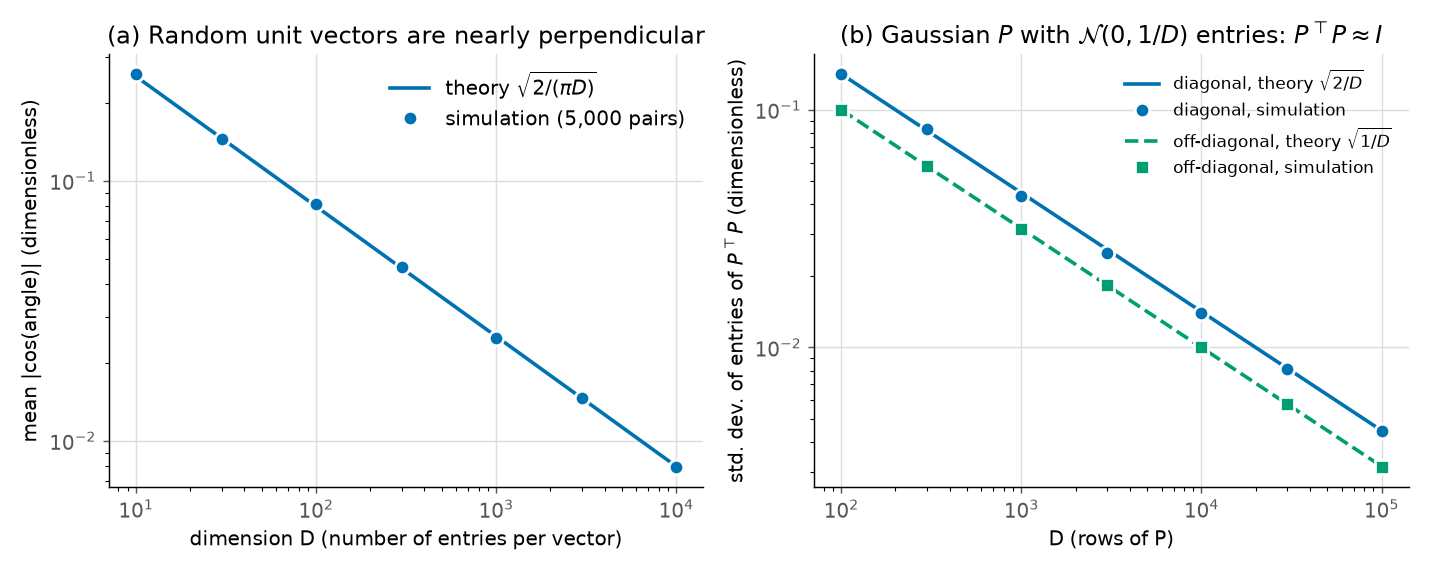
Figure: left, near-orthogonality of random unit vectors (output [7]); right, the spread of the entries of \(P^\top P\) around the identity for a Gaussian \(P\) (output [8]). Both axes are logarithmic, so a slope of \(-1/2\) means "shrinks like \(1/\sqrt D\)".
Going deeper¶
This chapter's proofs sit in collapsible blocks next to the facts they prove:
- associativity, the transpose of a product and Cauchy–Schwarz (under "Dot product and norm");
- lengths, angles and the trace argument for \(QQ^\top\ne I\) (under "Orthonormal columns");
- the "more unknowns than equations" lemma and \(\operatorname{rank}(BA)\le\min(\operatorname{rank}B,\operatorname{rank}A)\);
- every rank-\(\rho\) matrix factors as \(BA\);
- Gram–Schmidt works, and QR ignores scale;
- block transpose, block multiplication, the transpose rule and the mixed-product property;
- the vec trick, its row-stacking twin, and its cost;
- the variances \(1/D\), \(2/D\), \(1/D\) and the mean absolute cosine.
The block below combines them to compare the paper's two projector recipes.
Going deeper: the paper's two projectors through this chapter's tools
PAPER §3, p. 4 First recipe: \(P=(G_1\otimes G_2)/\sqrt D\), where \(G_1,G_2\) are \(\sqrt D\times\sqrt d\) matrices with independent \(\mathcal N(0,1)\) entries (the paper calls them \(Q_1,Q_2\)), "normalized so that" \(P^\top P\approx I\).
MY EXPLANATION By the transpose rule, the mixed-product property, and moving scalars freely,
SOURCE: Lotfi et al. 2022, §4.1 The same factorization appears there, with the conclusion \(P^\top P=I+O(D^{-1/4})\).
MY EXPLANATION Why \(D^{-1/4}\): each factor \(G_i^\top G_i/\sqrt D\) equals \(\tilde G_i^\top\tilde G_i\) with \(\tilde G_i=G_i/D^{1/4}\), a Gaussian matrix with only \(\sqrt D\) rows and entries of variance \(1/\sqrt D\). That is the setting of the near-orthogonality result with \(\sqrt D\) in place of \(D\). So the entries of each factor deviate from the identity by about \(1/\sqrt{\sqrt D}=D^{-1/4}\). Writing each factor as \(I+E_i\), the product is \(I\otimes I+E_1\otimes I+I\otimes E_2+E_1\otimes E_2\), so the total deviation is of the same order. The Kronecker structure saves memory but slows the approach to orthonormality: a dense Gaussian matrix with \(D\) rows deviates by about \(D^{-1/2}\). At a toy size (\(D=900\), \(d=25\)) the largest deviation of the first recipe is 0.81 (output [3]). Chapter 18 tracks it as \(D\) grows.
PAPER §5, p. 6 Second recipe: \(P=Q_1\otimes Q_2\), where \(Q_1,Q_2\) are the \(Q\)-factors of QR factorizations of \(\sqrt D\times\sqrt d\) Gaussian matrices.
MY EXPLANATION By the corollary, \(P^\top P=I\) exactly (output [3]: \(7.8\times10^{-16}\), rounding only). By the vec trick, \(Pw\) costs \(d\sqrt D+D\sqrt d\) multiplications, and \(P\) needs only \(2\sqrt D\sqrt d\) stored numbers, or just a seed.
[SOURCE: authors' code, sublora_nn_projectors.py] The released code takes QR factors of standard-normal
matrices (LazyRandomQR, used inside RoundedDoubleKronQR), i.e. the second recipe.
Paper erratum E08: two projector recipes, and an ambiguous N(0, 1/√D)
PAPER §3, p. 4; §5, p. 6 §3 describes Gaussian Kronecker factors scaled by \(1/\sqrt D\) with \(P^\top P\approx I\). §5 describes QR-orthogonalized factors, which give \(P^\top P=I\) exactly, and writes the Gaussian matrices as \(\mathcal N(0,1/\sqrt D)^{\sqrt D\times\sqrt d}\) without saying whether \(1/\sqrt D\) is a variance or a standard deviation.
MY EXPLANATION The two recipes give different matrices; the explainer follows §5, which is what the authors' code does. The variance-or-standard-deviation question does not matter for §5: QR returns the same \(Q\) whatever the scale of the Gaussian matrix ("Scale does not matter", above). Read as a variance, \(1/\sqrt D\) is the scale at which a Gaussian matrix with \(\sqrt D\) rows is already nearly orthonormal before QR; QR then removes the remaining deviation.
Paper erratum E37: Q, P and R change meaning between §3 and §5
PAPER §3, p. 4; §5, p. 6 In §3, \(Q_1,Q_2\) are raw Gaussian matrices. In §5, \(Q_1,Q_2\) are the orthonormal QR factors, while the raw Gaussian matrices are called \(P_1,P_2\) (reusing \(P\), already the projector and, in §4, the prior \(P(h)\)), and the triangular factor \(R_1\) in "\(Q_1R_1=P_1\)" reuses \(R\), the risk.
MY EXPLANATION No number changes, but a reader comparing §3 with §5 may think the same matrices are meant. This explainer writes \(G_1,G_2\) for raw Gaussian matrices, \(Q_1,Q_2\) for factors with orthonormal columns and \(T\) for triangular factors.
Common misconceptions¶
- Misconception: "\(P^\top P=I\) means \(P\) can be undone, so \(PP^\top=I\) as well." — Actually: for a tall \(D\times d\) matrix with \(d<D\), \(PP^\top\) is never the identity: its trace is \(d\), not \(D\). In the \(3\times2\) example its diagonal is \((5/9,5/9,8/9)\). \(P\) keeps lengths on the way into the big space, but most points of the big space are not of the form \(Pw\).
- Misconception: "The Kronecker product is a kind of ordinary matrix product, or an entry-by-entry product." — Actually: it multiplies every entry of \(M_1\) with every entry of \(M_2\), needs no matching sizes, and produces a bigger matrix of shape \((a_1a_2)\times(b_1b_2)\). Two \(2\times2\) matrices give a \(4\times4\) matrix.
- Misconception: "Low rank means small entries, or mostly zeros." — Actually: rank counts independent directions. \(\begin{pmatrix}1&10\\2&20\\3&30\end{pmatrix}\) has no zero entry and rank 1; the identity matrix is mostly zeros and has full rank.
- Misconception: "A product of an \(a\times r\) and an \(r\times b\) matrix always has rank exactly \(r\)." — Actually: at most \(r\). Random Gaussian factors gave rank 4 for \(r=4\), but repeating one column of \(B\) gave rank 3 (output [4]).
- Misconception: "A big random Gaussian matrix has orthonormal columns." — Actually: only approximately, with errors of size about \(1/\sqrt D\) (largest entry error 0.009 at \(D=100{,}000\), \(d=20\)). QR makes the columns orthonormal up to rounding (\(\sim10^{-16}\)). This is the difference between "≈" in §3 and "=" in §5 (erratum E08).
- Misconception: "Kronecker structure by itself makes \(P^\top P=I\)." — Actually: only if both factors have orthonormal columns (the corollary). With Gaussian factors scaled by \(1/\sqrt D\) but not orthogonalized, a \(900\times25\) example deviates by 0.81 (output [3]).
- Misconception: "To multiply by a Kronecker product you must first build it." — Actually: the vec trick uses only the two factors. At \(D=10^6\), \(d=10^4\) that is 0.80 MB of factors instead of a 40.0 GB matrix.
Self-test¶
Q1. A weight matrix has shape \(1024\times1024\). How many numbers does a rank-8 factorization \(BA\) store, and how many times fewer is that than the full matrix? What is the largest rank \(BA\) can have?
Answer
\(B\) is \(1024\times8\) and \(A\) is \(8\times1024\), so they hold \(8\cdot(1024+1024)=16{,}384\) numbers. The full matrix has \(1024\cdot1024=1{,}048{,}576\) entries, so the factorization is 64 times smaller (output [4]). The rank of \(BA\) is at most 8, because \(\operatorname{rank}(BA)\le\operatorname{rank}B\le8\) (\(B\) has only 8 columns). It can be less than 8 if the factors are degenerate, for example if two columns of \(B\) are equal.
Q2. \(Q\in\mathbb R^{9\times4}\) has orthonormal columns. True or false, with a reason: (a) \(\lVert Qw\rVert=\lVert w\rVert\) for every \(w\in\mathbb R^4\); (b) \(QQ^\top=I_9\); (c) \(\lVert Q^\top y\rVert=\lVert y\rVert\) for every \(y\in\mathbb R^9\).
Answer
(a) True: \(\lVert Qw\rVert^2=w^\top Q^\top Qw=w^\top w=\lVert w\rVert^2\).
(b) False: \(\operatorname{trace}(QQ^\top)=\operatorname{trace}(Q^\top Q)=\operatorname{trace}(I_4)=4\), while \(\operatorname{trace}(I_9)=9\).
(c) False. \(Q^\top y=0\) is a system of 4 equations in 9 unknowns, so by Lemma A ("more unknowns than equations") it has a solution \(y\ne0\). For that \(y\), \(\lVert Q^\top y\rVert=0\ne\lVert y\rVert\). Going "down" from the big space to the small one loses whatever is perpendicular to all columns of \(Q\).
Q3. You draw two independent random unit vectors in \(\mathbb R^{10{,}000}\). How large is their cosine typically, and what angle is that? How does the typical cosine change at \(D=100\)?
Answer
The cosine has mean 0 and variance exactly \(1/D\), so its standard deviation is \(1/\sqrt{10{,}000}=0.01\). A cosine of 0.01 is an angle of \(\arccos(0.01)=89.43\)° (output [7]). The average absolute cosine is about \(\sqrt{2/(\pi D)}=0.0080\) (simulated: 0.0079). At \(D=100\) the standard deviation is \(1/\sqrt{100}=0.1\), ten times larger (simulated: 0.1021): random directions are still close to perpendicular, but less so.
Code for this chapter¶
Run it from the project root (it takes under a minute on a laptop CPU):
.venv/Scripts/python explainer/code/ch08_linalg.py
Source: ch08_linalg.py
"""Chapter 8 demo -- linear-algebra toolkit.

Claims reproduced / checked (every number quoted in Chapter 8 is printed here):
  [1] small worked examples: a matrix-vector product and its cost, a rank-1 product,
      a matrix with orthonormal columns (Q^T Q = I and ||Qw|| = ||w||, but Q Q^T != I).
  [2] the Kronecker product M1 (x) M2 for M1 = [[1,2],[3,4]], M2 = [[0,1],[1,0]], the shape
      rule, and the vec trick (M1 (x) M2) vec(X) = vec(M2 X M1^T) on the same example.
  [3] the transpose rule and the mixed-product property on random matrices, and the corollary
      the paper relies on (§5, p. 6): if Q1, Q2 have orthonormal columns, then
      (Q1 (x) Q2)^T (Q1 (x) Q2) = I exactly.
  [4] rank(BA) <= r for LoRA-shaped factors (B 768x4, A 4x768); parameter counts r(a+b) vs ab.
  [5] QR: our Gram-Schmidt vs numpy (Householder) on a Gaussian 1000x50 matrix, plus an
      ill-conditioned matrix on which classical Gram-Schmidt loses orthogonality.
  [6] the vec trick at scale: P = Q1 (x) Q2 with D = 10^6, d = 10^4 applied without ever
      forming P; memory and multiplication counts.
  [7] near-orthogonality of random unit vectors: mean |cos| vs sqrt(2/(pi D)), std vs 1/sqrt(D).
  [8] a Gaussian D x d matrix with N(0, 1/D) entries: Var of diagonal entries of P^T P = 2/D,
      Var of off-diagonal entries = 1/D.
Figure: explainer/docs/assets/fig/ch08_near_orthogonal.png
Deterministic (numpy default_rng seeds); CPU only; runs in a few seconds.
"""
from __future__ import annotations

import sys
import time
from pathlib import Path

import numpy as np
import matplotlib

matplotlib.use("Agg")
import matplotlib.pyplot as plt  # noqa: E402

HERE = Path(__file__).resolve().parent
sys.path.insert(0, str(HERE))
import pacbound  # noqa: E402

OUT_TXT = HERE / "outputs" / "ch08_linalg.txt"
OUT_FIG = HERE.parent / "docs" / "assets" / "fig" / "ch08_near_orthogonal.png"

_lines: list[str] = []


def out(s: str = "") -> None:
    print(s)
    _lines.append(s)


# ---------------------------------------------------------------------------
# helpers
# ---------------------------------------------------------------------------
def vec(X: np.ndarray) -> np.ndarray:
    """Column stacking: first column of X on top, then the second column, ..."""
    return X.reshape(-1, order="F")


def unvec(v: np.ndarray, rows: int, cols: int) -> np.ndarray:
    """Inverse of vec: refill a rows x cols matrix column by column."""
    return v.reshape(rows, cols, order="F")


def kron_apply(Q1: np.ndarray, Q2: np.ndarray, w: np.ndarray) -> np.ndarray:
    """(Q1 (x) Q2) w computed as vec(Q2 X Q1^T) with X = unvec(w); never forms Q1 (x) Q2."""
    X = unvec(w, Q2.shape[1], Q1.shape[1])
    return vec(Q2 @ X @ Q1.T)


def gram_schmidt(G: np.ndarray):
    """Classical Gram-Schmidt exactly as described in the chapter.
    Returns Q (orthonormal columns) and T (upper triangular, positive diagonal) with G = Q T."""
    a, b = G.shape
    Q = np.zeros((a, b))
    T = np.zeros((b, b))
    for j in range(b):
        v = G[:, j].copy()
        for i in range(j):
            T[i, j] = Q[:, i] @ G[:, j]      # length of g_j along q_i
            v -= T[i, j] * Q[:, i]           # remove that part
        T[j, j] = np.linalg.norm(v)          # what is left, measured
        Q[:, j] = v / T[j, j]                # rescaled to length 1
    return Q, T


def orth_err(Q: np.ndarray) -> float:
    """max |entry of Q^T Q - I| (dimensionless)."""
    return float(np.max(np.abs(Q.T @ Q - np.eye(Q.shape[1]))))


def rows_str(M: np.ndarray, indent: str, width: int = 3) -> list[str]:
    return [indent + "[" + " ".join(f"{x:g}".rjust(width) for x in r) + " ]" for r in M]


def vec_str(v: np.ndarray, nd: int = 4) -> str:
    return "(" + ", ".join(f"{x:.{nd}g}" for x in v) + ")"


# ---------------------------------------------------------------------------
out("== Chapter 8: linear-algebra toolkit ==")

# [1] small worked examples ---------------------------------------------------
out("[1] small examples")
W = np.array([[1, 2], [3, 4], [5, 6]], dtype=float)
v = np.array([2, 1], dtype=float)
Wv = W @ v
assert np.array_equal(Wv, [4, 10, 16])
out(f"    W (3x2) = [[1,2],[3,4],[5,6]], v = (2, 1):  Wv = {vec_str(Wv)};  "
    f"multiplications = {W.shape[0] * W.shape[1]}")
b1 = np.array([[1], [2], [3]], dtype=float)
a1 = np.array([[1, 10]], dtype=float)
BA1 = b1 @ a1
assert np.linalg.matrix_rank(BA1) == 1
out(f"    (3x1)(1x2) product: [[1],[2],[3]] [[1,10]] = {BA1.astype(int).tolist()};  "
    f"rank = {np.linalg.matrix_rank(BA1)}")
u3, v3 = np.array([1.0, 2.0, 2.0]), np.array([2.0, 1.0, -2.0])
assert u3 @ v3 == 0 and np.linalg.norm(u3) == 3.0
out(f"    u = (1, 2, 2), v = (2, 1, -2):  u.v = {u3 @ v3:g},  ||u|| = {np.linalg.norm(u3):g},"
    f"  ||v|| = {np.linalg.norm(v3):g}")
Qs = np.array([[1, 2], [2, 1], [2, -2]], dtype=float) / 3.0
ws = np.array([3.0, 4.0])
Qw = Qs @ ws
assert orth_err(Qs) < 1e-15 and abs(np.linalg.norm(Qw) - 5.0) < 1e-14
QQt = Qs @ Qs.T
out("    Q = [[1,2],[2,1],[2,-2]]/3:  max|Q^T Q - I| = "
    f"{orth_err(Qs):.1e};  w = (3, 4), ||w|| = {np.linalg.norm(ws):g}")
out(f"    Qw = (11, 10, -2)/3 = {vec_str(Qw)},  ||Qw|| = {np.linalg.norm(Qw):.12g}")
out(f"    but Q Q^T != I: its diagonal is {vec_str(np.diag(QQt), 4)} "
    f"(= 5/9, 5/9, 8/9), trace = {np.trace(QQt):.12g}")

# [2] Kronecker example and vec trick ----------------------------------------
out("[2] Kronecker product example")
M1 = np.array([[1, 2], [3, 4]], dtype=float)
M2 = np.array([[0, 1], [1, 0]], dtype=float)
K = np.kron(M1, M2)
expected = np.array([[0, 1, 0, 2], [1, 0, 2, 0], [0, 3, 0, 4], [3, 0, 4, 0]], dtype=float)
assert np.array_equal(K, expected)
out("    M1 = [[1,2],[3,4]], M2 = [[0,1],[1,0]],  M1 (x) M2 =")
for s in rows_str(K, "      "):
    out(s)
shape = np.kron(np.ones((3, 2)), np.ones((4, 5))).shape
assert shape == (12, 10)
out(f"    shape rule: (3x2) (x) (4x5) -> {shape[0]}x{shape[1]}")
w4 = np.array([1, 2, 3, 4], dtype=float)
direct = K @ w4
X4 = unvec(w4, 2, 2)
trick = vec(M2 @ X4 @ M1.T)
assert np.array_equal(direct, trick) and np.array_equal(direct, [10, 7, 22, 15])
out(f"    w = (1,2,3,4): (M1(x)M2) w = {vec_str(direct)};  X = unvec(w) = {X4.astype(int).tolist()},"
    f" vec(M2 X M1^T) = {vec_str(trick)}")
out(f"    multiplications: direct {K.size}, trick {2 * 2 * 2} + {2 * 2 * 2} = {2 * 2 * 2 * 2}"
    " (no saving at this tiny size)")

# [3] identities on random matrices -------------------------------------------
out("[3] identities on random matrices (max abs error, float64)")
rng = np.random.default_rng(0)
A1, A2 = rng.standard_normal((3, 4)), rng.standard_normal((2, 5))
N1, N2 = rng.standard_normal((4, 3)), rng.standard_normal((5, 2))
e_t = float(np.max(np.abs(np.kron(A1, A2).T - np.kron(A1.T, A2.T))))
e_mp = float(np.max(np.abs(np.kron(A1, A2) @ np.kron(N1, N2) - np.kron(A1 @ N1, A2 @ N2))))
assert e_t == 0.0 and e_mp < 1e-12
out(f"    transpose rule  (M1(x)M2)^T = M1^T(x)M2^T, M1 3x4, M2 2x5:      {e_t:.1e}")
out(f"    mixed product   (M1(x)M2)(N1(x)N2) = (M1N1)(x)(M2N2), 6x20 by 20x6: {e_mp:.1e}")
Q1s, _ = np.linalg.qr(rng.standard_normal((30, 5)))
Q2s, _ = np.linalg.qr(rng.standard_normal((30, 5)))
Ps = np.kron(Q1s, Q2s)
e_c = orth_err(Ps)
e_g = orth_err(np.kron(rng.standard_normal((30, 5)), rng.standard_normal((30, 5))) / 30.0)
assert e_c < 1e-12
out(f"    corollary: Q1, Q2 30x5 orthonormal columns, P = Q1(x)Q2 is {Ps.shape[0]}x{Ps.shape[1]}:"
    f" max|P^T P - I| = {e_c:.1e}")
out(f"    (for contrast, Gaussian factors scaled by 1/sqrt(D) = 1/30, no QR: {e_g:.2f})")

# [4] rank and parameter counts -----------------------------------------------
out("[4] rank of a product of thin factors; parameter counts")
B = rng.standard_normal((768, 4))
A = rng.standard_normal((4, 768))
rB, rA, rBA = (int(np.linalg.matrix_rank(M)) for M in (B, A, B @ A))
assert (rB, rA, rBA) == (4, 4, 4)
out(f"    B 768x4, A 4x768 (Gaussian): rank B = {rB}, rank A = {rA}, rank BA = {rBA}"
    f"  (BA is {(B @ A).shape[0]}x{(B @ A).shape[1]})")
Bdeg = B.copy()
Bdeg[:, 1] = Bdeg[:, 0]
rdeg = int(np.linalg.matrix_rank(Bdeg @ A))
assert rdeg == 3
out(f"    same, but column 2 of B replaced by column 1: rank BA = {rdeg}")
for a, b, r in [(768, 768, 1), (768, 768, 4), (1024, 1024, 8)]:
    dense, low = a * b, r * (a + b)
    out(f"    {a}x{b}, r = {r}: dense {dense:>9,} numbers vs r(a+b) = {low:>6,}"
        f"  ({dense / low:.1f}x fewer)")
assert 768 * 768 == 589_824 and 4 * (768 + 768) == 6_144 and 589_824 / 6_144 == 96.0
out(f"    paper's grids [PAPER App. E]: largest subspace dimension d = {max(pacbound.D_GRID):,};"
    f" LoRA ranks r in {pacbound.R_GRID}")

# [5] QR decomposition ----------------------------------------------------------
out("[5] QR decomposition G = Q T of a Gaussian 1000x50 matrix G")
G = rng.standard_normal((1000, 50))
Qn, Tn = np.linalg.qr(G)
Qg, Tg = gram_schmidt(G)
for name, Qx, Tx in [("numpy (Householder)", Qn, Tn), ("our Gram-Schmidt   ", Qg, Tg)]:
    eo = orth_err(Qx)
    er = float(np.max(np.abs(G - Qx @ Tx)))
    tri = bool(np.allclose(Tx, np.triu(Tx), atol=0))
    assert eo < 1e-12 and er < 1e-12 and tri
    out(f"    {name}: max|Q^T Q - I| = {eo:.1e}, max|G - QT| = {er:.1e}, T upper triangular: {tri}")
ii = np.arange(1, 13)[:, None]
jj = np.arange(1, 9)[None, :]
Hilb = 1.0 / (ii + jj - 1)                      # 12x8 Hilbert-type matrix: nearly dependent columns
e_gs_h = orth_err(gram_schmidt(Hilb)[0])
e_np_h = orth_err(np.linalg.qr(Hilb)[0])
assert e_np_h < 1e-12 and e_gs_h > 1e-6
out(f"    ill-conditioned 12x8 matrix 1/(i+j-1): Gram-Schmidt max|Q^T Q - I| = {e_gs_h:.1e},"
    f" numpy = {e_np_h:.1e}")
wq = rng.standard_normal(50)
out(f"    isometry with numpy's Q: ||w|| = {np.linalg.norm(wq):.10f}, ||Qw|| = "
    f"{np.linalg.norm(Qn @ wq):.10f}")

# [6] vec trick at scale ---------------------------------------------------------
out("[6] vec trick at scale: P = Q1 (x) Q2 with Q1, Q2 of shape 1000x100 (orthonormal columns)")
sD, sd = 1000, 100
D, d = sD * sD, sd * sd
Q1, _ = np.linalg.qr(rng.standard_normal((sD, sd)))
Q2, _ = np.linalg.qr(rng.standard_normal((sD, sd)))
w = rng.standard_normal(d)
t0 = time.perf_counter()
Pw = kron_apply(Q1, Q2, w)
t1 = time.perf_counter()
spot = rng.choice(D, size=5, replace=False)
spot_err = max(abs(Pw[k] - np.kron(Q1[k // sD], Q2[k % sD]) @ w) for k in spot)
iso_err = abs(np.linalg.norm(Pw) - np.linalg.norm(w))
assert spot_err < 1e-12 and iso_err < 1e-9 and Pw.shape == (D,)
dense_bytes = D * d * 4
fac_bytes = 2 * sD * sd * 4
mult_dense = D * d
mult_trick = sD * sd * sd + sD * sd * sD
out(f"    D = {D:,}, d = {d:,}; dense P would hold {D * d:,} numbers = "
    f"{dense_bytes / 1e9:.1f} GB in float32 (1 GB = 1e9 bytes)")
out(f"    the two factors hold {2 * sD * sd:,} numbers = {fac_bytes / 1e6:.2f} MB"
    f"  ({dense_bytes / fac_bytes:,.0f}x less memory)")
out(f"    multiplications for Pw: dense {mult_dense:.2e}, trick {sD * sd * sd:.1e} + {sD * sd * sD:.1e}"
    f" = {mult_trick:.2e}  ({mult_dense / mult_trick:.0f}x fewer)")
out(f"    5 entries checked against rows of Q1(x)Q2: max error {spot_err:.1e};"
    f"  | ||Pw|| - ||w|| | = {iso_err:.1e}")
assert t1 - t0 < 5.0
print(f"    (wall time of the trick on this machine: {1e3 * (t1 - t0):.0f} ms; not written to the output file)")
out("    wall time of the trick: under 5 s (asserted; the exact time is machine-dependent, so it is not recorded)")

# [7] near-orthogonality of random unit vectors ----------------------------------
out("[7] two independent random unit vectors in R^D: cos(angle) = u.v (5,000 pairs per D)")
out("        D   mean|cos|  sqrt(2/(pi D))   std(cos)  1/sqrt(D)")
Ds_cos = [10, 30, 100, 300, 1000, 3000, 10000]
mean_abs, stds = [], []
n_pairs, chunk = 5000, 250
for Dk in Ds_cos:
    cos_all = []
    for _ in range(n_pairs // chunk):
        g = rng.standard_normal((chunk, Dk))
        h = rng.standard_normal((chunk, Dk))
        u = g / np.linalg.norm(g, axis=1, keepdims=True)
        vv = h / np.linalg.norm(h, axis=1, keepdims=True)
        cos_all.append(np.sum(u * vv, axis=1))
    c = np.concatenate(cos_all)
    ma, sdv = float(np.mean(np.abs(c))), float(np.std(c))
    th_ma, th_sd = float(np.sqrt(2 / (np.pi * Dk))), float(1 / np.sqrt(Dk))
    assert abs(ma / th_ma - 1) < 0.05 and abs(sdv / th_sd - 1) < 0.05
    mean_abs.append(ma)
    stds.append(sdv)
    out(f"    {Dk:>5}   {ma:.4f}     {th_ma:.4f}         {sdv:.4f}    {th_sd:.4f}")
ang = float(np.degrees(np.arccos(1 / np.sqrt(10000))))
out(f"    typical angle at D = 10,000: arccos(1/sqrt(D)) = arccos(0.01) = {ang:.2f} degrees")

# [8] Gaussian matrix with N(0, 1/D) entries ---------------------------------------
dg, reps = 20, 100
out(f"[8] Gaussian P (D x {dg}, entries N(0, 1/D)): entries of P^T P over {reps} draws")
out("         D   var(diag)    2/D       var(off)    1/D      max|P^T P - I| (one draw)")
Ds_g = [100, 300, 1000, 3000, 10000, 30000, 100000]
sd_diag, sd_off = [], []
iu = np.triu_indices(dg, k=1)
for Dk in Ds_g:
    diag_s, off_s, first_max = [], [], None
    for rep in range(reps):
        Pg = rng.standard_normal((Dk, dg)) / np.sqrt(Dk)
        S = Pg.T @ Pg
        diag_s.append(np.diag(S))
        off_s.append(S[iu])
        if rep == 0:
            first_max = float(np.max(np.abs(S - np.eye(dg))))
    vd = float(np.var(np.concatenate(diag_s)))
    vo = float(np.var(np.concatenate(off_s)))
    assert abs(vd / (2 / Dk) - 1) < 0.15 and abs(vo / (1 / Dk) - 1) < 0.15
    sd_diag.append(np.sqrt(vd))
    sd_off.append(np.sqrt(vo))
    out(f"    {Dk:>6}   {vd:.2e}   {2 / Dk:.2e}   {vo:.2e}   {1 / Dk:.2e}   {first_max:.3f}")

# figure ---------------------------------------------------------------------------
BLUE, ORANGE, GREEN, GREY = "#0072B2", "#D55E00", "#009E73", "#555555"
plt.rcParams.update({"font.size": 11})
fig, (ax1, ax2) = plt.subplots(1, 2, figsize=(11, 4.4))
Dl = np.logspace(1, 4, 200)
ax1.loglog(Dl, np.sqrt(2 / (np.pi * Dl)), color=BLUE, lw=2, label=r"theory $\sqrt{2/(\pi D)}$")
ax1.loglog(Ds_cos, mean_abs, "o", color=BLUE, ms=8, mec="white", mew=1.5,
           label="simulation (5,000 pairs)")
ax1.set_xlabel("dimension D (number of entries per vector)")
ax1.set_ylabel(r"mean $|\cos(\mathrm{angle})|$ (dimensionless)")
ax1.set_title("(a) Random unit vectors are nearly perpendicular")
ax1.grid(True, which="major", color="#dddddd", lw=0.8)
ax1.legend(frameon=False)
Dl2 = np.logspace(2, 5, 200)
ax2.loglog(Dl2, np.sqrt(2 / Dl2), color=BLUE, lw=2, label=r"diagonal, theory $\sqrt{2/D}$")
ax2.loglog(Ds_g, sd_diag, "o", color=BLUE, ms=8, mec="white", mew=1.5, label="diagonal, simulation")
ax2.loglog(Dl2, np.sqrt(1 / Dl2), color=GREEN, lw=2, ls="--", label=r"off-diagonal, theory $\sqrt{1/D}$")
ax2.loglog(Ds_g, sd_off, "s", color=GREEN, ms=8, mec="white", mew=1.5, label="off-diagonal, simulation")
ax2.set_xlabel("D (rows of P)")
ax2.set_ylabel(r"std. dev. of entries of $P^\top P$ (dimensionless)")
ax2.set_title(r"(b) Gaussian $P$ with $\mathcal{N}(0,1/D)$ entries: $P^\top P \approx I$")
ax2.grid(True, which="major", color="#dddddd", lw=0.8)
ax2.legend(frameon=False, fontsize=9.5)
for ax in (ax1, ax2):
    for side in ("top", "right"):
        ax.spines[side].set_visible(False)
    ax.tick_params(colors=GREY)
fig.tight_layout()
OUT_FIG.parent.mkdir(parents=True, exist_ok=True)
fig.savefig(OUT_FIG, dpi=130)
out("figure: explainer/docs/assets/fig/ch08_near_orthogonal.png")

OUT_TXT.parent.mkdir(parents=True, exist_ok=True)
OUT_TXT.write_text("\n".join(_lines) + "\n", encoding="utf-8")
Output:
== Chapter 8: linear-algebra toolkit ==
[1] small examples
    W (3x2) = [[1,2],[3,4],[5,6]], v = (2, 1):  Wv = (4, 10, 16);  multiplications = 6
    (3x1)(1x2) product: [[1],[2],[3]] [[1,10]] = [[1, 10], [2, 20], [3, 30]];  rank = 1
    u = (1, 2, 2), v = (2, 1, -2):  u.v = 0,  ||u|| = 3,  ||v|| = 3
    Q = [[1,2],[2,1],[2,-2]]/3:  max|Q^T Q - I| = 1.1e-16;  w = (3, 4), ||w|| = 5
    Qw = (11, 10, -2)/3 = (3.667, 3.333, -0.6667),  ||Qw|| = 5
    but Q Q^T != I: its diagonal is (0.5556, 0.5556, 0.8889) (= 5/9, 5/9, 8/9), trace = 2
[2] Kronecker product example
    M1 = [[1,2],[3,4]], M2 = [[0,1],[1,0]],  M1 (x) M2 =
      [  0   1   0   2 ]
      [  1   0   2   0 ]
      [  0   3   0   4 ]
      [  3   0   4   0 ]
    shape rule: (3x2) (x) (4x5) -> 12x10
    w = (1,2,3,4): (M1(x)M2) w = (10, 7, 22, 15);  X = unvec(w) = [[1, 3], [2, 4]], vec(M2 X M1^T) = (10, 7, 22, 15)
    multiplications: direct 16, trick 8 + 8 = 16 (no saving at this tiny size)
[3] identities on random matrices (max abs error, float64)
    transpose rule  (M1(x)M2)^T = M1^T(x)M2^T, M1 3x4, M2 2x5:      0.0e+00
    mixed product   (M1(x)M2)(N1(x)N2) = (M1N1)(x)(M2N2), 6x20 by 20x6: 1.8e-15
    corollary: Q1, Q2 30x5 orthonormal columns, P = Q1(x)Q2 is 900x25: max|P^T P - I| = 7.8e-16
    (for contrast, Gaussian factors scaled by 1/sqrt(D) = 1/30, no QR: 0.81)
[4] rank of a product of thin factors; parameter counts
    B 768x4, A 4x768 (Gaussian): rank B = 4, rank A = 4, rank BA = 4  (BA is 768x768)
    same, but column 2 of B replaced by column 1: rank BA = 3
    768x768, r = 1: dense   589,824 numbers vs r(a+b) =  1,536  (384.0x fewer)
    768x768, r = 4: dense   589,824 numbers vs r(a+b) =  6,144  (96.0x fewer)
    1024x1024, r = 8: dense 1,048,576 numbers vs r(a+b) = 16,384  (64.0x fewer)
    paper's grids [PAPER App. E]: largest subspace dimension d = 200,000; LoRA ranks r in [1, 4]
[5] QR decomposition G = Q T of a Gaussian 1000x50 matrix G
    numpy (Householder): max|Q^T Q - I| = 8.9e-16, max|G - QT| = 5.8e-15, T upper triangular: True
    our Gram-Schmidt   : max|Q^T Q - I| = 5.6e-16, max|G - QT| = 2.7e-15, T upper triangular: True
    ill-conditioned 12x8 matrix 1/(i+j-1): Gram-Schmidt max|Q^T Q - I| = 1.0e+00, numpy = 4.4e-16
    isometry with numpy's Q: ||w|| = 8.4270394012, ||Qw|| = 8.4270394012
[6] vec trick at scale: P = Q1 (x) Q2 with Q1, Q2 of shape 1000x100 (orthonormal columns)
    D = 1,000,000, d = 10,000; dense P would hold 10,000,000,000 numbers = 40.0 GB in float32 (1 GB = 1e9 bytes)
    the two factors hold 200,000 numbers = 0.80 MB  (50,000x less memory)
    multiplications for Pw: dense 1.00e+10, trick 1.0e+07 + 1.0e+08 = 1.10e+08  (91x fewer)
    5 entries checked against rows of Q1(x)Q2: max error 1.1e-16;  | ||Pw|| - ||w|| | = 1.4e-14
    wall time of the trick: under 5 s (asserted; the exact time is machine-dependent, so it is not recorded)
[7] two independent random unit vectors in R^D: cos(angle) = u.v (5,000 pairs per D)
        D   mean|cos|  sqrt(2/(pi D))   std(cos)  1/sqrt(D)
       10   0.2577     0.2523         0.3139    0.3162
       30   0.1454     0.1457         0.1820    0.1826
      100   0.0814     0.0798         0.1021    0.1000
      300   0.0466     0.0461         0.0582    0.0577
     1000   0.0249     0.0252         0.0313    0.0316
     3000   0.0146     0.0146         0.0184    0.0183
    10000   0.0079     0.0080         0.0100    0.0100
    typical angle at D = 10,000: arccos(1/sqrt(D)) = arccos(0.01) = 89.43 degrees
[8] Gaussian P (D x 20, entries N(0, 1/D)): entries of P^T P over 100 draws
         D   var(diag)    2/D       var(off)    1/D      max|P^T P - I| (one draw)
       100   2.00e-02   2.00e-02   1.00e-02   1.00e-02   0.280
       300   6.83e-03   6.67e-03   3.39e-03   3.33e-03   0.195
      1000   1.89e-03   2.00e-03   9.96e-04   1.00e-03   0.091
      3000   6.22e-04   6.67e-04   3.35e-04   3.33e-04   0.048
     10000   1.95e-04   2.00e-04   1.00e-04   1.00e-04   0.027
     30000   6.60e-05   6.67e-05   3.31e-05   3.33e-05   0.017
    100000   1.99e-05   2.00e-05   9.88e-06   1.00e-05   0.009
figure: explainer/docs/assets/fig/ch08_near_orthogonal.png